Do you think IIT Guwahati certified course can help you in your career?
Introduction
In graph theory, finding the shortest path between two vertices is a fundamental problem, often solved using algorithms like Dijkstra’s or Bellman-Ford. However, in certain scenarios, we may want to maximize the shortest path between two given vertices by adding a single edge to the graph. This approach can help improve the overall connectivity and efficiency of the network.
In this article, we will explore the concept of maximizing the shortest path by adding a single edge, its applications, and step-by-step methods to achieve this optimization.
Problem statement
In the problem, you are given an undirected graph with ‘V’ vertices numbered from 1 to ‘V’ and ‘E’ edges between these ‘V’ vertices also you are given with an array named as operation of ‘K’ size which store ‘K’ number of vertices and you are allowed to join an edge between any two vertices given in the array and by making these connections. Your task is to maximize the shortest path between the first and the last vertex.
Note: You may add an edge between any two selected vertices that have already an edge between them to maximize the shortest path.
Example
Input
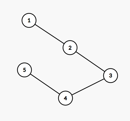
An unweighted graph is given with 5 vertices named as 1, 2, 3, 4, 5, and 4 edges between (1-2),(2-3),(3-4), and (4-5). The value of K here is 3 and the operation array is given as {1, 2, 4}. We have to maximize the shortest path by adding a single edge between the combinations of all the possible vertices in the operation array.
So let’s explore all the possible combinations of vertices in the operation array
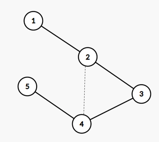
Considering edge 2, 4 from the operation array, the shortest distance between 1 and 5 here is 3
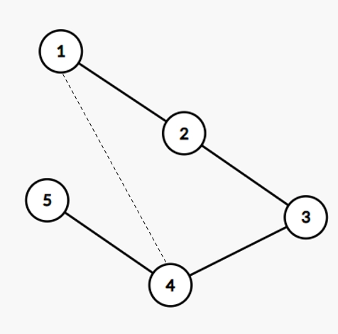
Considering the edge 1, 4 from the operation array, the shortest distance between 1 and 5 here is 2
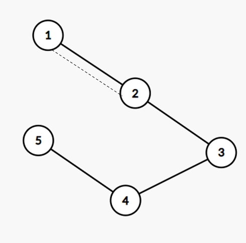
Considering the edge 1, 2 from the operation array the shortest distance between 1 and 5 here is 4
Out of all these possible shortest distances, we have to maximize the shortest path or shortest distance. So the maximum of all the shortest distance that is max(2, 3, 4) is 4 so the answer for this graph is 4 units
Approach
This problem of maximize the shortest path can be solved in the series of steps as follows :
The idea here is to calculate the minimum distance for every vertex from the first and the last vertex
Let the shortest distance for a random vertex v from first node be xv and from the last vertex be yv
For this, maintain a 2D matrix having 2 rows and v columns to store the minimum distance of all the vertices from the starting vertex in the first row and from the last vertex in the second row
Now, choose two operation vertices a and b from operation[] array to minimize the value of min(xa + yb, ya + xb)
Let distance = min(xa + yb, ya + xb)
Fro minimizing this distance follow these rules
Create a vector of pairs and store the value of (xv - yv) with their respective selected vertex and after storing all the values sort the vector of pairs
Before traversing in the vector initialize the value of best to 0 and max to -INF
Now traverse the above vector of pairs and for each selected node(say n) update the value of best to maximum of (best, max + dist[1][n]) and update max to maximum of (max, dist[0][n]).
After the above operations the maximum of (dist[0][v-1] and best + 1) given the minimum shortest path which will ultimately solve the goal to maximize the shortest path
Code:
#include <bits/stdc++.h>
using namespace std;
const int INF = INT_MAX;
int v,e;

// To store graph as adjacency list
vector<int> graph[100000];

// To store the shortest path from first vertex and last vertex
int dist[2][100000];


// Bfs traversal of finding shortest distance from source vertex
void bfs(int* dist, int starting_vertex)
{

    int queue[200000];

    // Filling initially each distance as infinity
    fill(dist, dist + v, INF);

    int first = 0, second = 0;
    queue[first++] = starting_vertex;
    dist[starting_vertex] = 0;

    // Performing BFS
    while (second < first) {

        int x = queue[second++];

        for (int y : graph[x]) {
            if (dist[y] == INF) {

                // Updating the distance and queue
                dist[y] = dist[x] + 1;
                queue[first++] = y;
            }
        }
    }
}

/*
    Function that maximise the shortest path between source and destination
    vertex by adding a single edge between given selected nodes
*/

void shortestPathCost(int operation[], int K)
{
    vector<pair<int, int> > dp;

    // To update the shortest distance between node 1 to other vertices
    bfs(dist[0], 0);

    // To update the shortest distance between node N to other vertices
    bfs(dist[1], v - 1);

    for (int i = 0; i < K; i++) {


        // Storing the values  of (x[i] - y[i])
        dp.push_back({dist[0][operation[i]]
                            - dist[1][operation[i]],
                        operation[i]});
    }


    sort(dp.begin(), dp.end());
    int best = 0;
    int MAX = -INF;

    // Traversing  dp array
    for (auto it : dp) {
        int a = it.second;
        best = max(best,
                MAX + dist[1][a]);

        /*
             Maximise the value of (x[a] - y[b]) if a and b
             are the current vertices in operations
       */
        MAX= max(MAX, dist[0][a]);
    }

    // Printing the minimum cost
    cout<<min(dist[0][v - 1], best + 1);

}

int main()
{

    //Given total vertices and edges and operation array to choose edges
    v = 5, e = 4;
    int K = 2;
    int operation[] = { 1, 2 ,4};

    // Sorting the nodes in operation
    sort(operation, operation + K);

    // Formation of graph
    graph[0].push_back(1);
    graph[1].push_back(0);
    graph[1].push_back(2);
    graph[2].push_back(1);
    graph[2].push_back(3);
    graph[3].push_back(2);
    graph[3].push_back(4);
    graph[4].push_back(3);

    // maximise the shortest path

    shortestPathCost(operation, K);
    return 0;
}
You can also try this code with Online C++ Compiler
The time complexity for the solution of “maximize the shortest path” will be O(V * log V + E) where ‘V’ is the number of vertices and ‘E’ is the number of edges so let's understand the time complexity for the given problem.
First we have to sort the array operation that will cost us (K * log K ) for using inbuilt sort function
Second we are entering in shortestPathCost function here we are calling bfs for first vertex which will cost us (V + E) and again for last vertex which will cost ( V + E ) so the time complexity for these 2 bfs calls will be 2 * ( V + E) and simultaneously we are also storing the shortest distance in the dp array of size V then we are sorting the dp array which will cost V * log V
So the total time complexity after all the operations will be:
(K * log K ) + 2 * (V + E) + V * log V
Here K is very small compared with V so neglect the factor of K in the driver code now the complexiy will become
2 * (V + E) + V * log V
V * (log V + 2 ) + E
~ O(V * log V + E)
Space Complexity
The space complexity for the problem “maximize the shortest path” is O(N) since we are using a vector of pairs to store (xv – yv) here ‘xv’ is the shortest distance of a particular vertex ‘V’ from the first node and similarly ‘yv’ is shortest distance for the same vertex from the last node
Frequently Asked Questions
How is Dijkstra different from normal BFS?
Dijkstra and BFS are two different algorithms for calculating the shortest distance between two points. Dijkstra's approach is based on a priority queue, whereas regular bfs are based on a queue. we can use either of these algorithms to solve the above problem maximize the shortest path
How to find the shortest path in the weighted graph?
There are two most famous algorithms for finding the shortest distance in the weighted graph that is using Bellman-Ford in O(VE). If there are no negative weight cycles we can also use the Dijkstra algorithm that will do the work for us in O(E + VLogV)
Different ways to store graphs?
We can use an adjacency list, adjacency matrix, there is one more way here we can store Nodes as objects and edges as pointers.
Conclusion
In this blog, we solved the problem “maximize the shortest path” that is maximizing the shortest distance between the first vertex and last vertex in the graph by adding a single edge from the operation array given.


 8+ registered

