MLE in statistical models
Conditional MLE for a supervised learning model can be given as:-
Maximise{∑(i to n) log P(xi ; h)}
Where h is the modelling hypothesis which replaces the model parameters. ‘h’ can be any supervised learning model we’re trying to optimise.
Maximum Likelihood Estimation in Logistic Regression
The objective here would be to predict the best sigmoid curve for the given observation. And for that we need to find the best parameters. For that, we’ll use MLE.
Let the required cost function be given by P(Y;z). Where Y is our sample data and z is the unknown parameter.
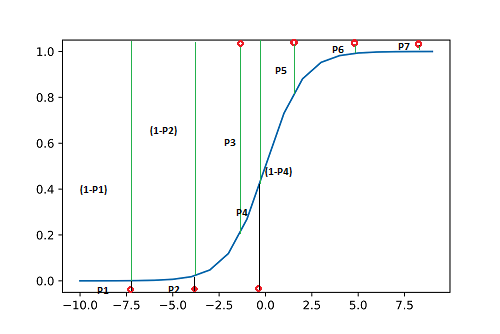
Source - link
Here, we have 7 points with respective probabilities their respective probabilities. For points to be 0 we need P1, P2, P4 to be as low as possible and for points to be 1, we need probabilities P3, P5, P6 and P7 to be as high as possible.
This may also be restated as if we need the product
(1-P1)*(1-P2)* P3*(1-P4)*P5*P6*P7
to be maximized. This is called the joint probability. The cost function may be written as-
J(z) = π(i to n) P (Yi ; z) (for n samples)
ln J(z) = ln(π(i to n) P (Yi ; z)) (Taking natural logs)
ln J(z) =L(z|Yi) = ∑(i to n) ln P (Yi ; z))
For a given value of z and the corresponding sample Yi, the function gives the probability of obtaining the observed values. If Yi=1 ,function becomes z. For Yi=0, the function becomes 1-z.
ln J(z) =L(z|Yi)= ∑(i to n) ln (zyi *(1-z)1-yi ))
Simplifying it further, the final expression comes out to be-
The function maximizes at z= ∑(i=1 to n) Yi/n
Implementation
# import the necessary libraries
import numpy as np
import pandas as pd
from matplotlib import pyplot as plt
import seaborn as sns
from statsmodels import api
from scipy import stats
from scipy.optimize import minimize

You can also try this code with Online Python Compiler
# create an independent variable
x = np.linspace(-10, 30, 100)
# create a normally distributed residual
e = np.random.normal(10, 5, 100)
# generate ground truth
y = 10 + 4*x + e
df = pd.DataFrame({'x':x, 'y':y})
df.head()
You can also try this code with Online Python Compiler

# visualize data distribution
sns.regplot(x='x', y='y', data = df)
plt.show()
You can also try this code with Online Python Compiler

BY OLS APPROACH
features = api.add_constant(df.x)
model = api.OLS(y, features).fit()
model.summary()
You can also try this code with Online Python Compiler

# find the std dev
res = model.resid
standard_dev = np.std(res)
standard_dev
You can also try this code with Online Python Compiler

BY MLE APPROACH
def MLE_Norm(parameters):
  const, beta, std_dev = parameters
  pred = const + beta*x

  LL = np.sum(stats.norm.logpdf(y, pred, std_dev))
  neg_LL = -1*LL
  return neg_LL
You can also try this code with Online Python Compiler
mle_model = minimize(MLE_Norm, np.array([2,2,2]), method='L-BFGS-B')
mle_model
You can also try this code with Online Python Compiler

The parameters obtained via both the approaches are similar.
Frequently Asked Questions
Contrast Maximum likelihood estimation with ordinary least squares in linear regression.
The MLE chooses parameters that can maximize the likelihood or, equivalently the log-likelihood function. It then fits the model based on the trial estimated parameter value and calculate the mean of the model. To find the iterative weighted and working dependence and based on this two and the design matrix we can estimate the best parameter value.
OLS checks and minimizes the residual errors(square of the difference between observed value and the predicted value) of the model.
Provide an expression for maximum likelihood estimation in linear regression.
Without getting too much into the derivation, the final expression can be given as
Maximize {∑(i to n) log (1 / √(2 *π*sigma2)) – (1/(2 *sigma2) * (yi – h(xi, Beta))2)}
xi is a given example and beta is the coefficients of the linear regression model.
State the advantages of MLE over other estimators.
Following are the advantages of MLE over other estimators:
→ If model assumptions are right, it is the most efficient parameter estimation technique.
→ Provides a flexible approach suitable for a variety of applications.
→ Works the best for larger samples.
Conclusion
Maximum likelihood estimation is a popular and widely used optimisation technique among data scientists. Maximum likelihood estimation chooses parameters in such a way that it maximizes the likelihood of observing the datapoints. Although, most companies might not expect a beginner to be aware of the nitty-gritty of this technique, an extra bit of knowledge always goes a long way. You may check out our industry-oriented machine learning courses curated by industry experts.


 6+ registered

