Do you think IIT Guwahati certified course can help you in your career?
Introduction
Many of us would have come across the term gradient descent while studying the optimization techniques in machine learning. Optimization plays a crucial role in playing with data sets and finding the model with the best accuracy showcasing better results.
Gradient descent does the same by finding a local minimum of the differential function of the data set. Further, the gradient descent is divided into three more sub-categories from which mini-batch gradient descent is one such optimization technique we would learn in this article.
Before learning about the mini-batch gradient descent, let's have a quick flashback of the essentials that are necessary to understand the functioning of mini-batch gradient descent and the reason for its use.
Gradient Descent
Gradient descent, as discussed earlier, is an optimization technique used to optimize the accuracy of models by finding the best practical value of parameters known as coefficients of a function used to minimize the cost function. Gradient descent mathematically can be described as
Let's understand this formula with the help of the diagram given below.
As shown in the above plot, any random point on the blue surface is called the coefficients of the current value from the training data set.
The bottom-most point that we can see in red is the best set of coefficients, also known as the minimum function and the goal of using gradient descent is to find the best possible value of coefficient that provides the optimum cost of the cost function that evaluates the overall performance of our model.
Types of Gradient Descent
Batch Descent
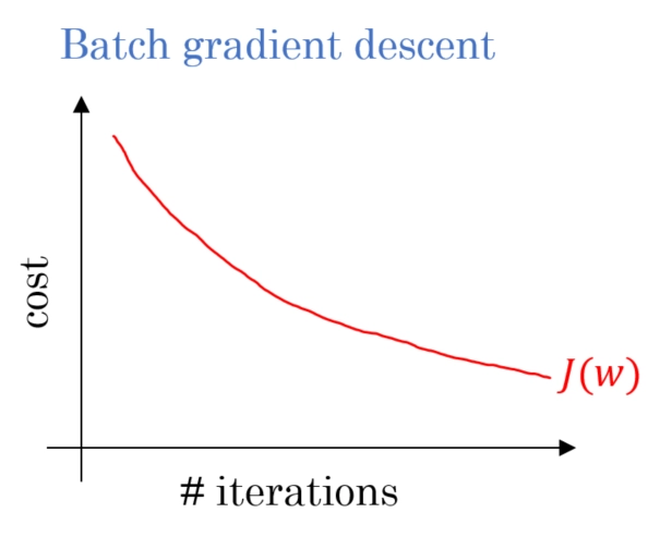
While using Batch gradient descent, we go through all the given data points in our dataset and calculate the cumulative error in a single step or a single epoch. The graph of the batch gradient descent is smooth and has less noise.
The average of all the data points, along with the cumulative error, is used to optimize the given dataset for our model. The mean gradient is used to update the parameters.
Stochastic Descent
The Stochastic gradient descent, unlike batch gradient, doesn't go through all the samples; instead, it picks one random parameter and optimizes the dataset according to the recorded value of data points that makes learning happen at every update.
The graph of stochastic gradient descent contains noise as the parameters are taken randomly, which causes disturbance in the graph.
Mini-Batch Descent
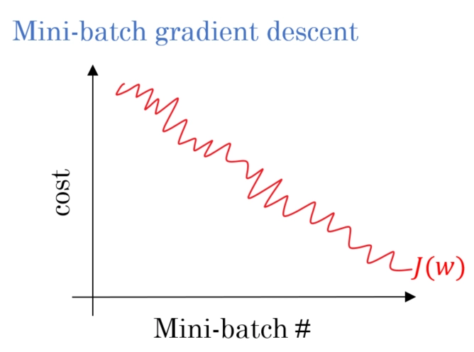
Instead of going through the complete dataset or choosing one random parameter, Mini-batch gradient descent divides the entire dataset into randomly picked batches and optimizes it.
The graph of mini-batch gradient descent is something in between the batch gradient descent and stochastic gradient descent as it contains more noise than batch gradient descent but less noise than stochastic gradient descent.
Comparison Table
Batch Descent
Stochastic Descent
Mini-Batch Descent
Uses all training samples while training the dataset and only after the complete cycle makes the required update in the training dataset.
It uses one random training sample and makes the required update in the training dataset.
Divides the dataset into batches and, after completion of every batch makes the required update in the dataset.
Requires too much time and computational space for one epoch.
Faster than Batch descent and requires moderate computational space.
It is the fastest and requires minimal computational space.
Best to use for small training datasets
Best for training big datasets with less computational requirement.
Best for large training datasets.
Mini-Batch Gradient Descent
We are already well-versed with the basics of mini-batch gradient descent now; let’s dive right in and explore in dept about mini-batch gradient descent.
Mini-batch gradient descent is a gradient descent modification that divides the training dataset into small batches that are used to compute model error and update model coefficients.
Implementations may opt to sum the gradient over the mini-batch, which minimizes the gradient's variance even further.
Mini-batch gradient descent attempts to achieve a value between the robustness of stochastic gradient descent and the efficiency of batch gradient descent. It is the most frequent gradient descent implementation used in regression techniques, neural networks, and deep learning.
Theoretically, in Mini- Batch Gradient descent, we move as follows:
We choose random data points and an initial learning rate.
In case the error keeps getting higher, reduce the learning rate
In case the error is fair but shows slow change, you can increase the learning rate.
With the help of minimal codes, we create a program to automate the rate of learning on the given dataset.
While reaching towards the last batch, one should decrease the learning rate as it helps reduce the noise and fluctuation in the data generated.
We tur down the learning rate once the error stops decreasing.
The algorithm used:
We take random parameters from the dataset along with a maximum number of epochs the optimization should take place.
Let theta = model parameters and max_iters = number of epochs.
We iterate the dataset to find the bias and the errors in the random parameters take
for itr = 1, 2, 3, …, max_iters:
We divide the dataset into mini-batches and iterate them to update the required values.
for mini_batch (X_mini, y_mini):
The update is made and in the batches, the prediction is made.
Predict the batches X_mini:
Let’s understand the implementation of mini-batch gradient descent with the help of code.
Code for mini-batch gradient descent
Step1: Let’s import our dataset from sklearn and check the number of rows and input columns.
from sklearn.datasets import load_diabetes
import numpy as np
from sklearn.linear_model import LinearRegression
from sklearn.metrics import r2_score
from sklearn.model_selection import train_test_split
X,y = load_diabetes(return_X_y=True)
print(X.shape)
print(y.shape)
You can also try this code with Online Python Compiler
Step 5: Create a class and ask for a batch parameter to divide the given data set into batches.
#Import random module to pick random data points.
import random
class MBGDRegressor:
   #Take input of the batch size.
    def __init__(self,batch_size,learning_rate=0.01,epochs=100):

        #Create class size attributes.
        self.coef_ = None
        self.intercept_ = None
        self.lr = learning_rate
        self.epochs = epochs
        self.batch_size = batch_size
  #Apply the fit method where change the intercept to 0 and all the attributes to 1.
    def fit(self,X_train,y_train):
        # init your coefs
        self.intercept_ = 0
        self.coef_ = np.ones(X_train.shape[1])

        for i in range(self.epochs):
            #This loop would work according to the batch size given.
            for j in range(int(X_train.shape[0]/self.batch_size)):

                idx = random.sample(range(X_train.shape[0]),self.batch_size)

                y_hat = np.dot(X_train[idx],self.coef_) + self.intercept_
                intercept_der = -2 * np.mean(y_train[idx] - y_hat)
                self.intercept_ = self.intercept_ - (self.lr * intercept_der)
                coef_der = -2 * np.dot((y_train[idx] - y_hat),X_train[idx])
                self.coef_ = self.coef_ - (self.lr * coef_der)
        print(self.intercept_,self.coef_)

    def predict(self,X_test):
        return np.dot(X_test,self.coef_) + self.intercept_
You can also try this code with Online Python Compiler
Step 8: Use sklearn model to describe the final batch size and partial fit for the dataset.
from sklearn.linear_model import SGDRegressor
sgd = SGDRegressor(learning_rate='constant',eta0=0.1)
batch_size = 35
for i in range(100):
    idx = random.sample(range(X_train.shape[0]),batch_size)
    sgd.partial_fit(X_train[idx],y_train[idx])
sgd.coef_
You can also try this code with Online Python Compiler
Step 9: Print the intercept of the given linear regression found after the update made on the model after training it with the randomly chosen data points.
sgd.intercept_
You can also try this code with Online Python Compiler
We can use different ways to speed up the algorithm of the mini-batch gradient, but in this section, we will be discussing only the most popular ones.
Momentum
Instead of changing the parameter’s position in the given dataset by gradient descent in momentum instead of the position, we change the velocity.
RMSprop
This method divides the learning rate for parameters by a running average of the coefficients of recent gradients for that parameter.
Adam Optimization
The adam optimization and the implementation of momentum and RMSprop introduce the bias correction, which further helps speed up the optimization.
Frequently Asked Questions
Q1. What are the limitations of gradient descent?
Ans: The particular drawback of gradient descent is It can take a long time to reach a local minimum of the given dataset. There is no guarantee that the technique will locate the global minimum if there are many local minima.
Q2. Is it necessary to use mini-batch gradient descent on big datasets?
Ans: The mini-batch gradient descent approach divides the training dataset into small batches that are used to calculate model error and update model coefficients. Implementations may choose to sum the gradient throughout the mini-batch, which minimizes the gradient's variance even further, making the optimization easier.
Q3.How many batches do we make in the gradient descent?
Ans: The number of batches the dataset is divided into depends on the user and the model one is working with, as the randomness of the data plays a crucial role in deciding the given factor.
Key Takeaways
Gradient descent has wide application in machine learning, neural networks, and deep learning. Gradient descent minimizes the loss function of a model. Mini-batch gradient descent helps reduce the loss function by randomly choosing the data points and dividing them into batches making the update after the complete computation of one batch, making computation easy and the optimization fast.
This article has also seen the basics of gradient descent and its types; to learn more about similar machine learning techniques, follow our blogs and explore more.


 9+ registered

