What is convergence failure in a generative adversarial network?

A failure to converge means not finding an equilibrium between the discriminator and the generator.

What happens to the generator at the convergence failure?

The generator is expected to produce highly low-quality images identified as fake by the discriminator.

How can we identify model collapse in GANs?

The generator model is expected to generate identical output images from different points in the latent space

What are the ways to impair the stable GAN?

Changing the Adam optimization algorithm to be too aggressiveUsing very large or petite kernel sizes in the models.

Table of contents

Introduction

Ways To Tackle Model Collapse

Implementation

FAQs

Key Takeaways

Last Updated: Mar 27, 2024

Model Collapse in GANs

Author Rajkeshav

Do you think IIT Guwahati certified course can help you in your career?

Yes

Introduction

GANs are a prevalent class of deep layer models, an example of an implicit problem model; that is, a model where we are defining a Sampling procedure.

source

In GANs, we essentially have this process, and we will effectively draw some random vectors from the standard Gaussian. Then we will feed that into a determinant transformation parametrized by theta, a neural network, so that's usually called a generator. Then we will take the output of the neural network as the sample from our distribution. The fundamental idea of GANs is to introduce classifiers known as the discriminator and try to train them to differentiate between actual data and examples. And then, our goal is to teach the generator to fool the discriminator. One of the critical problems with GANs is that we can have mode collapse.

source

We have taken a simple one-dimensional setting where, for example, the data is coming from the shown distribution. The model may only capture one of the modes of the data distribution, so it may forget or ignore that this is the part of the data. Now, how serious is this problem? Google does a paper, and they studied how bad mode collapse is, and then it turns out even for the best GANs, we can drop 72% of the mode. They did this study on the synthetic data set where precision and recall can be precisely computed. The other exciting thing to notice is that this GAN that achieves the best recall level is the original GAN. The other ones are essentially the later improvements.

Why does mode collapse happen?

source

Here we have simple two-dimensional data. Here the red squares are the actual data examples, and the blue circles are generated samples. When we train GAN on this data set, we will prepare the discriminator in the first step.

source

In this case, we have one nearest neighbour classifier. The Yellow regions correspond with the area where the discriminator thinks that the thing is real, and the White region is where things are fake. The objective for the generator is to try to portrait all these blue circles that the generator samples to the yellow area.

source

After one random training, we train the generator to have all the blue circles in the yellow region. We will prepare the discriminator to differentiate between blue circles and red squares and a new decision boundary. We will train the generator again, and all the blue circles will go to the yellow region.

source

And that is what we get after two rounds of training, and we can notice that here at the top right corner, there are the red squares that don't have any blue Circles. So these are the form modes that the generator is not capturing. Why did this happen? If we think back to what just happened, we essentially pushed all these different generator samples, that is, the blue circles, towards the nearest data example. This ensures that the generated model is a nearby data example, but it does not guarantee a nearby generated sample.

Also See, Resnet 50 Architecture

Ways To Tackle Model Collapse

We can tackle modal collapse in GANs by following approaches.

Grouping the classes empowers the discriminator to discriminate against sub-batches to determine if a given batch is real or fake.
Anticipating counter action removes the situation of the discriminator chasing the generator by training the generator to fool the discriminator maximally.
Learning from experience involves training the discriminator on the fake data generated by the generator in a given number of rounds.
Multiple networks involve training multiple generative networks for each class and covering all the data classes.

Implementation

Training an unstable GAN for generating handwritten digits

1. Mention the size of the latent space

latent_dim = 1

2. Import necessary libraries

from os import makedirs
from numpy import expand_dims
from numpy import zeros
from numpy import ones
from numpy.random import randn
from numpy.random import randint
from keras.datasets.mnist import load_data
from keras.optimizers import Adam
from keras.models import Sequential
from keras.layers import Dense
from keras.layers import Reshape
from keras.layers import Flatten
from keras.layers import Conv2D
from keras.layers import Conv2DTranspose
from keras.layers import LeakyReLU
from keras.initializers import RandomNormal
from matplotlib import pyplot

3. Building the discriminator model

def define_discriminator(in_shape=(28,28,1)):
# weight initialization
init = RandomNormal(stddev=0.02)
# define model
model = Sequential()
# downsample to 14x14
model.add(Conv2D(64, (4,4), strides=(2,2), padding='same', kernel_initializer=init, input_shape=in_shape))
model.add(LeakyReLU(alpha=0.2))
# downsample to 7x7
model.add(Conv2D(64, (4,4), strides=(2,2), padding='same', kernel_initializer=init))
model.add(LeakyReLU(alpha=0.2))
# classifier
model.add(Flatten())
model.add(Dense(1, activation='sigmoid'))
# compile model
opt = Adam(lr=0.0002, beta_1=0.5)
model.compile(loss='binary_crossentropy', optimizer=opt, metrics=['accuracy'])
return model

4. Building the generator model

def define_generator(latent_dim):
# weight initialization
init = RandomNormal(stddev=0.02)
# define model
model = Sequential()
# foundation for 7x7 image
n_nodes = 128 * 7 * 7
model.add(Dense(n_nodes, kernel_initializer=init, input_dim=latent_dim))
model.add(LeakyReLU(alpha=0.2))
model.add(Reshape((7, 7, 128)))
# upsample to 14x14
model.add(Conv2DTranspose(128, (4,4), strides=(2,2), padding='same', kernel_initializer=init))
model.add(LeakyReLU(alpha=0.2))
# upsample to 28x28
model.add(Conv2DTranspose(128, (4,4), strides=(2,2), padding='same', kernel_initializer=init))
model.add(LeakyReLU(alpha=0.2))
# output 28x28x1
model.add(Conv2D(1, (7,7), activation='tanh', padding='same', kernel_initializer=init))
return model

5. combine generator and discriminator model

def define_gan(generator, discriminator):
# make weights in the discriminator not trainable
discriminator.trainable = False
# connect them
model = Sequential()
# add generator
model.add(generator)
# add the discriminator
model.add(discriminator)
# compile model
opt = Adam(lr=0.0002, beta_1=0.5)
model.compile(loss='binary_crossentropy', optimizer=opt)
return model

6. You can use any data from an outside source, I am loading mnist images.

def load_real_samples():
# load dataset
(trainX, trainy), (_, _) = load_data()
# expand to 3d, e.g. add channels
X = expand_dims(trainX, axis=-1)
# select all of the examples for a given class
selected_ix = trainy == 8
X = X[selected_ix]
# convert from ints to floats
X = X.astype('float32')
# scale from [0,255] to [-1,1]
X = (X - 127.5) / 127.5
return X

7. Select the real samples

def generate_real_samples(dataset, n_samples):
# choose random instances
ix = randint(0, dataset.shape[0], n_samples)
# select images
X = dataset[ix]
# generate class labels
y = ones((n_samples, 1))
return X, y

8. Generate points in latent space as input for the generator

def generate_latent_points(latent_dim, n_samples):
# generate points in the latent space
x_input = randn(latent_dim * n_samples)
# reshape into a batch of inputs for the network
x_input = x_input.reshape(n_samples, latent_dim)
return x_input

9. Use the generator to generate n fake examples, with class labels

def generate_fake_samples(generator, latent_dim, n_samples):
# generate points in latent space
x_input = generate_latent_points(latent_dim, n_samples)
# predict outputs
X = generator.predict(x_input)
# create class labels
y = zeros((n_samples, 1))
return X, y

10. Generate samples and save as a plot and save the model

def summarize_performance(step, g_model, latent_dim, n_samples=100):
# prepare fake examples
X, _ = generate_fake_samples(g_model, latent_dim, n_samples)
# scale from [-1,1] to [0,1]
X = (X + 1) / 2.0
# plot images
for i in range(10 * 10):
# define subplot
pyplot.subplot(10, 10, 1 + i)
# turn off axis
pyplot.axis('off')
# plot raw pixel data
pyplot.imshow(X[i, :, :, 0], cmap='gray_r')
# save plot to file
pyplot.savefig('results_collapse/generated_plot_%03d.png' % (step+1))
pyplot.close()
# save the generator model
g_model.save('results_collapse/model_%03d.h5' % (step+1))

11. Create a line plot of loss for the gan and save to file

def plot_history(d1_hist, d2_hist, g_hist, a1_hist, a2_hist):
# plot loss
pyplot.subplot(2, 1, 1)
pyplot.plot(d1_hist, label='d-real')
pyplot.plot(d2_hist, label='d-fake')
pyplot.plot(g_hist, label='gen')
pyplot.legend()
# plot discriminator accuracy
pyplot.subplot(2, 1, 2)
pyplot.plot(a1_hist, label='acc-real')
pyplot.plot(a2_hist, label='acc-fake')
pyplot.legend()
# save plot to file
pyplot.savefig('results_collapse/plot_line_plot_loss.png')
pyplot.close()

12. Train the Generator and Discriminator

def train(g_model, d_model, gan_model, dataset, latent_dim, n_epochs=10, n_batch=128):
# calculate the number of batches per epoch
bat_per_epo = int(dataset.shape[0] / n_batch)
# calculate the total iterations based on batch and epoch
n_steps = bat_per_epo * n_epochs
# calculate the number of samples in half a batch
half_batch = int(n_batch / 2)
# prepare lists for storing stats each iteration
d1_hist, d2_hist, g_hist, a1_hist, a2_hist = list(), list(), list(), list(), list()
# manually enumerate epochs
for i in range(n_steps):
# get randomly selected 'real' samples
X_real, y_real = generate_real_samples(dataset, half_batch)
# update discriminator model weights
d_loss1, d_acc1 = d_model.train_on_batch(X_real, y_real)
# generate 'fake' examples
X_fake, y_fake = generate_fake_samples(g_model, latent_dim, half_batch)
# update discriminator model weights
d_loss2, d_acc2 = d_model.train_on_batch(X_fake, y_fake)
# prepare points in latent space as input for the generator
X_gan = generate_latent_points(latent_dim, n_batch)
# create inverted labels for the fake samples
y_gan = ones((n_batch, 1))
# update the generator via the discriminator's error
g_loss = gan_model.train_on_batch(X_gan, y_gan)
# summarize loss on this batch
print('>%d, d1=%.3f, d2=%.3f g=%.3f, a1=%d, a2=%d' %
(i+1, d_loss1, d_loss2, g_loss, int(100*d_acc1), int(100*d_acc2)))
# record history
d1_hist.append(d_loss1)
d2_hist.append(d_loss2)
g_hist.append(g_loss)
a1_hist.append(d_acc1)
a2_hist.append(d_acc2)
# evaluate the model performance every 'epoch'
if (i+1) % bat_per_epo == 0:
summarize_performance(i, g_model, latent_dim)
plot_history(d1_hist, d2_hist, g_hist, a1_hist, a2_hist)

13. Make folder for results and create the models

makedirs('results_collapse', exist_ok=True)
latent_dim = 1
discriminator = define_discriminator()
generator = define_generator(latent_dim)
gan_model = define_gan(generator, discriminator)
dataset = load_real_samples()
print(dataset.shape)

14. Train the model

train(generator, discriminator, gan_model, dataset, latent_dim)

Output

Line plot for loss and accuracy of GAN With a convergence failure due to lot of Aggressive Optimisation

FAQs

What is convergence failure in a generative adversarial network?
A failure to converge means not finding an equilibrium between the discriminator and the generator.
What happens to the generator at the convergence failure?
The generator is expected to produce highly low-quality images identified as fake by the discriminator.
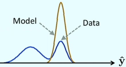
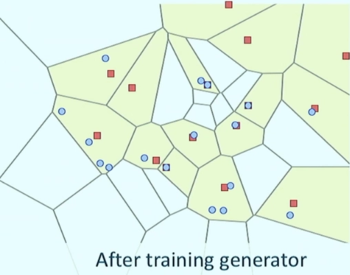
How can we identify model collapse in GANs?
The generator model is expected to generate identical output images from different points in the latent space
What are the ways to impair the stable GAN?
Changing the Adam optimization algorithm to be too aggressive
Using very large or petite kernel sizes in the models.
Which part of machine learning is a generative adversarial network?
Unsupervised learning

Key Takeaways

In this tutorial, we looked at the model collapse in generative adversarial networks and how to tackle it along with the code implementation. Visit Machine Learning to explore more about similar exciting models.

Further readings-

Face Detection

N-Gram Modelling

Rolling and Unrolling RNN