Motion Estimation using Optical Flow

Different Optical Flow Algorithms

There are different Optical Flow Algorithms, such as:

Horn-Schunck Method

This method helps us in tracking movement in videos. It analyses specific points or attributes in an image and then examines how they move from one frame to another.The Brightness Constancy Assumption assumes that the lighting does not change from one frame to another.  

This method believes that the movement in the frame is very small. The algorithm studies how the brightness changes in these points and uses that to figure out the direction and speed of the moving object. People use this method in real-time, like tracking objects in surveillance, robots, and augmented reality (AR) applications. However, it might only work well with small movements and not in complicated situations where many things block the view.

Farneback Method

The Farneback algorithm determines how each Pixel moves from one frame to another in a picture or a video. It smartly estimates the motion using a maths formula representing the Pixel change. This method efficiently calculates and handles big or small motions in a video. It breaks down the frames into smaller frames and then accurately determines the direction and amount of movement for every Pixel. It allows us to understand the motion and differences in the images or videos.

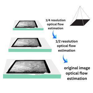
Pyramid Optical Flow

Pyramid Optical Flow is a way to find and determine how objects move in a picture or a video. It determines this by analyzing different versions of the images generated at various sizes. It helps to identify significant and small movements more accurately. First, it checks a fuzzy part to spot large movements. 

Then, it switches to a more transparent part to identify smaller movements and finer details. In this way, it handles complex parts very well. Although you can find optical flow using different algorithms, Pyramid optical flow is recommended as it helps you quickly identify complex motion.

FlowNet and Deep Learning-based Methods

FlowNet and Deep Learning-based Methods are modern techniques used in computer vision to figure out how things move in pictures and videos. FlowNet is a particular type of deep learning system. It uses neural networks to learn motion patterns in an image or videos. It does not require any handwritten formulas. It identifies the optical flow from the raw data itself. The deep learning method uses deep neural networks for optical flow estimation.

Example of using Motion Estimation using Optical Flow

Let's take an example to understand Motion Estimation using Optical Flow. 

Code

# Import necessary libraries
import cv2
import numpy as np
from google. collab.patches import cv2_imshow

# Load the video
cn_cap = cv2.VideoCapture("/content/Coding_ninjas_video.mp4")

# Parameters for Lucas-Kanade optical flow
cn_lk_params = dict(winSize=(15, 15),
                    maxLevel=2,
                    criteria=(cv2.TERM_CRITERIA_EPS | cv2.TERM_CRITERIA_COUNT, 10, 0.03))

# Read the first frame and find initial points to track
cn_ret, cn_old_frame = cn_cap.read()
cn_old_gray = cv2.cvtColor(cn_old_frame, cv2.COLOR_BGR2GRAY)
cn_corners = cv2.goodFeaturesToTrack(cn_old_gray, maxCorners=100, qualityLevel=0.3, minDistance=7)
cn_mask = np.zeros_like(cn_old_frame)

# Define the codec 
cn_fourcc = cv2.VideoWriter_fourcc(*'XVID')
cn_out = cv2.VideoWriter('coding_ninjas_output.avi', cn_fourcc, 30.0, (cn_old_frame.shape[1], cn_old_frame.shape[0]))

while True:
    cn_ret, cn_frame = cn_cap.read()
    if not cn_ret:
        break
    cn_frame_gray = cv2.cvtColor(cn_frame, cv2.COLOR_BGR2GRAY)
   
    # Calculate optical flow using the Lucas-Kanade method
    cn_new_corners, cn_st, cn_err = cv2.calcOpticalFlowPyrLK(cn_old_gray, cn_frame_gray, cn_corners, None, **cn_lk_params)
    
    # Select good points
    cn_good_new = cn_new_corners[cn_st == 1]
    cn_good_old = cn_corners[cn_st == 1]
    
    # Draw the tracks on the image
    for i, (new, old) in enumerate(zip(cn_good_new, cn_good_old)):
        cn_a, cn_b = new.ravel()
        cn_c, cn_d = old.ravel()
        cn_a, cn_b = int(cn_a), int(cn_b) 
        cn_c, cn_d = int(cn_c), int(cn_d) 
        cn_mask = cv2.line(cn_mask, (cn_a, cn_b), (cn_c, cn_d), (0, 255, 0), 2)
        cn_frame = cv2.circle(cn_frame, (cn_a, cn_b), 5, (0, 255, 0), -1)
    cn_img = cv2.add(cn_frame, cn_mask)
    cn_out.write(cn_img) 
   
    # Write the frame to the output video
    cv2_imshow(cn_img)
    if cv2.waitKey(30) & 0xFF == ord('q'):
        break
   
    # Update the previous frame and points
    cn_old_gray = cn_frame_gray.copy()
    cn_corners = cn_good_new.reshape(-1, 1, 2)

# Release video capture
cn_cap.release()
cn_out.release()
cv2.destroyAllWindows()

Output

Output video

Explanation

In this code, we have used the Lucas-Kanade Optical Flow method to track the feature points in the video. First, we imported all the necessary libraries, like cv2, and loaded the video. We have defined parameters for Lucas-Kanade optical flow. Then we read the first frame and find the initial points for tracking. We have converted the image to grayscale for optical flow calculations. The output will be in frames, so I have transformed it into a video to understand the motion clearly. We have used the function "cv2.calcOpticalFlowPyrLK" to calculate the optical flow between the previous and current frames. We then trace the motion on the frame using green lines and circles to indicate the movement of these points.

Difference between Sparse Optical Flow and Dense Optical Flow

There are some differences between Sparse Optical Flow and Dense Optical Flow such as:

Applications of Motion Estimation Using Optical Flow 

There are many applications of Motion Estimation using Optical Flow, such as:

• Motion estimation helps in tracking moving objects in movies, enabling applications such as surveillance, augmented reality, and driverless cars to identify motion.
   
• Motion analysis algorithms generate intermediate frames in video interpolation and super-resolution, enhancing video quality and providing smooth slow-motion effects.
   
• Motion estimation is necessary for robotic systems because it permits robots to navigate and interact with their surroundings by identifying their movement and the movement of surrounding objects.
   
• Motion estimation is used in action recognition systems to evaluate and classify human movements in the video, which helps applications such as gesture recognition and human-computer interaction.
   
• In sports analytics, motion estimation algorithms follow players' movements and assess game dynamics, offering significant information for coaching and strategy development.

Challenges in Motion Estimation using Optical Flow

Some challenges involved in Motion Estimation using Optical Flow are:

• When objects experience complex motion patterns or occlusions, optical flow can become complicated and pixel displacements may be confusing.
   
• Changes in lighting conditions might cause feature matching to fail, making it challenging to estimate motion effectively using intensity-based approaches.
   
• Optical flow has difficulty figuring out movement in areas with very little or similar patterns because there are few clear signs to follow.
   
• When motion is perpendicular to the gradient, optical flow techniques may fail to accurately determine the direction of movement.
   
• High-resolution pictures and real-time applications require fast techniques for estimating optical flow while attaching to intense computing restrictions.

Frequently Asked Questions

What is Motion estimation?

Computer vision and video processing use the motion estimation technique to determine how things move from one frame to the next in a succession of photos or movies. It helps create video compression by tracking objects, examining their movement patterns, etc.

What are the principles of motion estimation?

The basic principles of motion estimation are comparing pixels from various frames and identifying patterns. This method repeats for several frames to trace the object's motion over time.

What function does motion estimation serve?

Estimating motion is essential for many applications. By comparing successive frames and determining changes, video compression can decrease the file size while preserving good-quality output.

Do alternative motion estimating techniques exist?

There are algorithms for estimating motion, like block-based and optical flow-based techniques. In the block-based approach, frames are divided into blocks and then compressed to find the motion vectors. In the optical flow method, the Pixel of a movement is analyzed to find the object's motion.

What difficulties does motion estimation face?

In some cases where recurring patterns, quick movements, or occlusion (where one object hides another) occur, determining accurate motion vectors can be difficult.

Conclusion

In this article, we learn about Motion Estimation using Optical Flow. We explore different algorithms used in motion estimation. With the help of an example, we learned how to estimate an object's motion. We even discussed the difference between spare and dense optical flow. Ultimately, we learned about the challenges of Motion estimation using optical flow.

Do check out the link to learn more about such topic

• Human-Computer Interaction
• Self-Driving Cars - Application of ML
• Application of Computer Vision

You can find more informative articles or blogs on our platform. You can also practice more coding problems and prepare for interview questions from well-known companies on your platform, Coding Ninjas Studio.