Must Know Functions in Scikit-Learn

Installation of Scikit-learn

To start using Scikit-learn, you first need to install it. Here are the steps to install Scikit-learn on your system:

1. Install Python (if not already installed):

• Scikit-learn requires Python version 3.7 or later. You can download Python from the official website: python.org.

2. Install pip (if not already installed):

• pip is the package installer for Python. It is usually included with Python installations. If you don't have it, you can install it by following the instructions on the official pip installation guide.

3. Install Scikit-learn using pip:

• Open your terminal (or command prompt) and run the following command: pip install scikit-learn

4. Verify the installation:

• After installation, verify that Scikit-learn is correctly installed by opening a Python interpreter and running:
  import sklearn
  print(sklearn.__version__)
• This will print the installed version of Scikit-learn, confirming that the installation was successful.

5. (Optional) Install additional dependencies:

• If you plan to work with advanced functionalities, you may need additional dependencies like numpy, scipy, or matplotlib. To install them, run: pip install numpy scipy matplotlib

Datasets

→ One of the significant functionality of sklearn is the availability of inbuilt datasets. 

→ Sklearn provides access to various inbuilt datasets such as the Iris Plants Dataset, Boston House Prices Dataset, Diabetes Dataset, Breast Cancer Dataset, and the MNIST Dataset. 

#loading Iris Dataset using sklearn
import pandas as pd
import sklearn
from sklearn import datasets
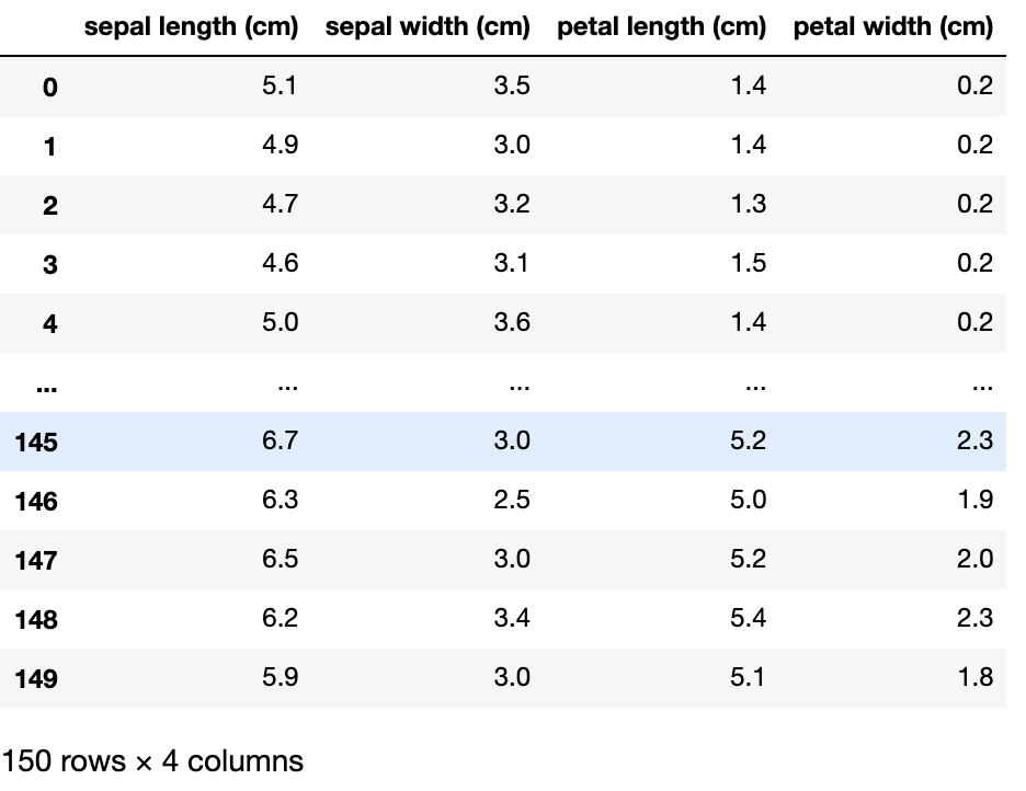
iris = datasets.load_iris()
df = pd.DataFrame(iris.data, columns=iris.feature_names)
df

Output

→ In the above code, we have imported the iris dataset and printed the dataframe of the same. 

→ Similarly, we can import other datasets and visualize them using sklearn. 

#boston dataset 
boston= datasets.load_boston()
#load_diabetes
diabetes= datasets.load_diabetes()

Preprocessing

→ Preprocessing is an essential component for making data training ready. 

(i) Standardization

→ Standardization of datasets is essential in the domain of Machine Learning. 

→ Individual features need to look more or less like standard normally distributed data. 

→ Standardization is essential, especially when a feature has a high magnitude variance compared to the other features. 

→ Sklearn provides ‘StandardScaler’ functionality in the ‘Preprocessing’ module. 

→ Standardization makes use of mean and standard deviation for scaling. 

#standard scaler 

from sklearn import preprocessing
import numpy as np
train_x = np.array([[ 1, -2,  1],[ 2,  1,  0], [ 0,  1, -1]])
scaler = preprocessing.StandardScaler().fit(train_x)

scaled_x = scaler.transform(train_x)
scaled_x

print(scaled_x.mean(axis=0))
print(scaled_x.std(axis=0))

Output

→ We notice that scaled data has its mean as zero and its variance as 1. 

→ An alternative standardization technique is to use ‘MinMaxScaler().’ This scales features in the range (min, max). This is usually between 0 and 1. 

(ii) Normalization

→ Normalization is a technique applied as part of data preparation in Machine Learning. 

→ It refers to transforming features for them to be on a similar scale. 

→ Normalization makes use of minimum and maximum values of features to perform scaling. 

→ We can perform this operation on a dataset using any of ‘l1’, ‘l2’, or ‘max’ norms. 

#Normalization

X = [[ 1, 2,  -1],[ 0,  2,  1], [ 1,  0, -1]]
X_normalized = preprocessing.normalize(X, norm='l2')
X_normalized

Output

(iii) Encoding

→ Label Encoding can be performed to convert categorical features to numerical features. 

→ This will ensure that everything is in machine-readable form. 

→ Machine learning algorithms can then decide how the labels must be operated in a better way. 

→ This step is essential in the case of Supervised Learning. 

#Label Encoding 

df= pd.read_csv('iris.csv')

#initial labels
print(df['Species'].unique())

label_encoder = preprocessing.LabelEncoder()
df['Species']= label_encoder.fit_transform(df['Species'])

#encoded labels
print(df['Species'].unique())

Output

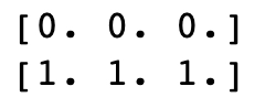
→ In the above output, we notice that initially, the labels were categorical. 

→ After performing label encoding using sklearn, we converted the features to numerical ones. 

→ One limitation of label encoding is that it assigns a unique integer to each label. This might cause priority issues or bias in our model. For example, Labels with high values may be considered to be of higher priority than labels with low values. 

→ ‘One hot encoding’ helps overcome this issue by converting a separate column for each unique label. For example, consider a dataset with the target variable as ‘Hair Colour.’ There are two unique labels, ‘black’ and ‘brown.’ If we predict ‘black,’ we will have ‘1’ in the ‘black’ column and ‘0’ in the ‘brown’ column and vice-versa.

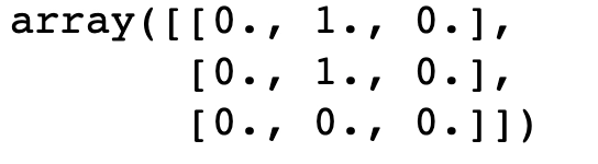
#one Hot encoding 

enc = preprocessing.OneHotEncoder()
X = [['male', 'Hindu', 'Chrome'], ['female', 'Sikh', 'Safari']]
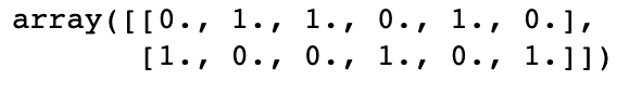
enc.fit(X)
enc.transform(X).toarray()

Output

→ In the above output, we notice a separate column for each unique label. These columns are filled with values ‘0’ or ‘1’, indicating the output at each input. 

(iv) Binarization

→ Binarization refers to thresholding numerical features to get boolean values. 

→ This technique is very common in the field of text processing. 

→ We can use the ‘Binarizer’ function for this technique. This function is part of the ‘Preprocessing’ module. 

#Binarizer 

X = [[ 1., 2.,  -1.], [ 0,  2.,  0.], [ 0.2,  1., -1.]]

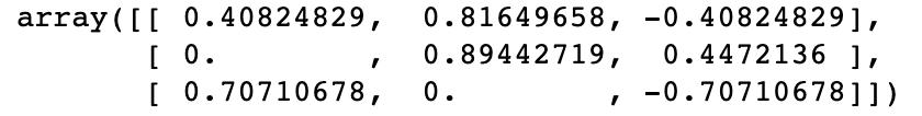
binarizer = preprocessing.Binarizer(threshold=1)  # fit does nothing
binarizer.transform(X)

Output

→ In the above code, we notice that using Binarizer, we set the threshold as 1. This implies that all those values >1 would be assigned a ‘1’ whereas those <=1 would be given a ‘0’. 

→ Hence, we have been able to binarize the given array. 

(v) Splitting 

→ We can use sklearn for splitting data into training data and testing data. 

#train-test split
from sklearn.model_selection import train_test_split

df= pd.read_csv('iris.csv')
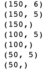
print(df.shape)

X= data [ : , 0:5]
Y= data [:, -1]

print(X.shape)
print(Y.shape)

#split
train_x, test_x, train_y, test_y = train_test_split(X, Y, test_size=50, random_state=4)

#printing shapes to check split
print(train_x.shape)
print(train_y.shape)
print(test_x.shape)
print(test_y.shape)

Output

→ In the above code, we have specified the test size as 50. As a result, we get the following shapes/dimensions:-

• Train_x : (100,5)
• Train_y : (100, )
• Test_x : (50, 5)
• Test_y : (50, )

Models

→ We can implement various models such as Linear Regression, Logistic Regression, Naive Bayes, Decision Trees, Random Forests, Support Vector Machines, KMeans, and more using none other than sklearn. 

(i) Linear Regression

#Linear Regression

from sklearn.linear_model import LinearRegression

regression_model = LinearRegression()

regression_model.fit(train_x, train_y)

y_predicted = regression_model.predict(test_x)

→ In the above code, we have created the Linear Regression model object. ‘LinearRegression()’ creates an object of Linear Regression. Then, we fit this model on the training set and then get the predictions on the test set. 

(ii) KMeans

→ We will test the KMeans model on the Iris Dataset and get the predictions. 

#KMeans
from sklearn.cluster import KMeans

kmeans = KMeans(n_clusters=3)
kmeans.fit(train_x, train_y)

# training predictions
train_labels= kmeans.predict(train_x)

#testing predictions
test_labels = kmeans.predict(test_x)

test_labels

Output

→ In the above code, we have applied KMeans on the Iris Dataset and generated the predictions for the same. 

→ Similarly, we can use sklearn for implementing other models. 

from sklearn.tree import DecisionTreeClassifier
from sklearn.ensemble import RandomForestClassifier
from sklearn import svm
from sklearn.cluster import DBSCAN

Results

→ As part of sklearn, various evaluation metrics are available for testing our models. 

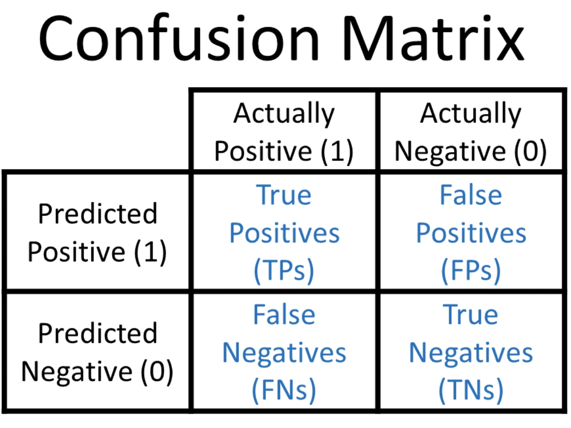
(i) Confusion Matrix

→ A confusion matrix is a table describing the performance of classification models. It consists of the following four terms:-

• True Positive(TF): the model predicted positive, and it is actually positive.

• True Negative(TN): the model predicted negative, and it is actually negative. 
• False Positive(FP): the model predicted positive, but it is actually negative. 
• False Negative(FN): the model predicted negative, but it is actually positive. 

from sklearn.metrics import confusion_matrix
confusion_matrix = confusion_matrix(y_test, y_pred)

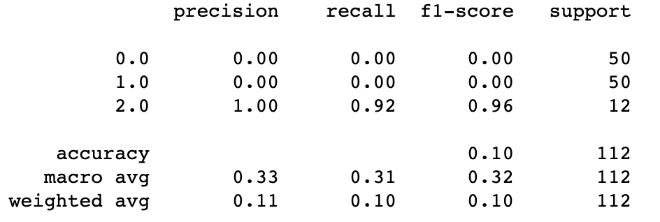
(ii) Classification Report

→ It helps to analyze the predictions of classification algorithms. 

→ It consists of various parameters:-

• Accuracy: number of correct predictions 

(TF+TN)/(TF+TN+FP+FN)*100

• Precision: number of correct positive predictions. 

TP/(TP+FP)

• Recall: number of correct predictions out of total positives. 

TP/(TP+FN)

• F1 Score: checks balance between precision and recall. 

2/(Precision + Recall)

#classification report for training set 
print(classification_report(train_y, train_labels))

Output

Frequently Asked Questions

Q1. Which Python libraries are essential for Machine Learning apart from sklearn?

Some of the other vital libraries are:-

• Scipy
• Theano
• TensorFlow
• Keras
• PyTorch
• Pandas
• Numpy
• Matplotlib

Q2. What is the difference between sklearn and scikit-learn?

Sklearn and Scikit-learn are two different names for the same library. sklearn is a dummy project on PyPi that will, in turn, install Scikit-learn.

Q3. What is the limitation of sklearn?

The limitation of sklearn is that it is not optimized for graph algorithms. It is not very suitable for string processing too.

Q4. Is sklearn a library or package?

Scikit-learn, often imported as sklearn, is a Python package that provides simple and efficient tools for data analysis and machine learning. It is a collection of modules and functions that work together to build predictive models and process data.

Conclusion

Scikit-learn is an invaluable tool for anyone working with machine learning in Python, offering a wide range of functions to simplify the entire process from data preprocessing to model evaluation. By mastering the essential functions discussed in this blog, you can significantly enhance your ability to build and optimize machine learning models.