NER with KERAS and Tensorflow

Introduction

We will use a Kaggle-provided NER dataset for this project. You can find the dataset here. This dataset is a subset of the GMB corpus, which has been tagged, annotated, and constructed specifically to train the classifier to predict named items such as name, location, and so on. One more characteristic (POS) is included in the dataset that can be utilized for categorization. However, in this project, we are only working with one feature sentence.

Importing Libraries

# importing libraries
import pandas as pd
from itertools import chain
from sklearn.model_selection import train_test_split
from keras.preprocessing.sequence import pad_sequences
from tensorflow.keras.utils import to_categorical
import numpy as np
import tensorflow
from tensorflow.keras import Sequential, Model, Input
from tensorflow.keras.layers import LSTM, Embedding, Dense, TimeDistributed, Dropout, Bidirectional
from tensorflow.keras.utils import plot_model
from numpy.random import seed
import spacy
from spacy import displacy

You can also try this code with Online Python Compiler

Run Code

Reading Dataset

I am training this model in google colab so to train the model in google colab we need to mount our drive.

from google.colab import drive
drive.mount('/content/drive/')
data = pd.read_csv('/content/drive/MyDrive/Datasets/ner_dataset.csv', encoding= 'unicode_escape')
data.head()

You can also try this code with Online Python Compiler

Run Code

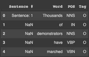
The sentences in the dataset are tokenized In the "Word" column. The "sentence #" column displays the sentence number once before printing NaN till the following sentence starts. Our label will be in the 'Tag' column (y).

Extracting Mappings

We'll utilize two mappings to train a neural network, as given below.

token to token_id: address the current token's row in the embeddings matrix.

tag to tag_id: one-hot ground truth probability distribution vectors for computing the loss at the network's output.

This phase is required in any machine learning model that accepts integers as input, such as the neural network.

def dictionary_map(data, tt):
   t2i = {}
   i2t = {}
  
   if tt == 'token':
       v = list(set(data['Word'].to_list()))
   else:
       v = list(set(data['Tag'].to_list()))
  
   i2t = {i:t for  i, t in enumerate(v)}
   t2i = {t:i for  i, t in enumerate(v)}
   return t2i, i2t


t2i, i2t = dictionary_map(data, 'token')
ta2i, i2ta = dictionary_map(data, 'tag')
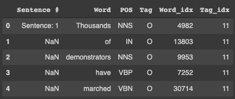
data['Word_idx'] = data['Word'].map(t2i)
data['Tag_idx'] = data['Tag'].map(ta2i)
data.head()

You can also try this code with Online Python Compiler

Run Code

For our X (Word idx) and y (Tag idx) variables, we can see that the function has introduced two additional index columns. To make the most of the recurrent neural network, let's collect tokens into arrays in the proper order.

Extract sequential data by transforming columns

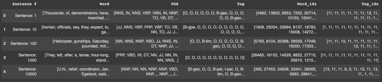
1. Fill NaN in the 'sentence #' column using method ffill in fillna to convert columns into sequential arrays.

2. Then, on the sentence column, run groupby to generate a list of tokens and tags.

# filling all the NAN values
dfn = data.fillna(method='ffill', axis=0)

# Groupby & collect columns
dgrp = dfn.groupby(
['Sentence #'],as_index=False
)['Word', 'POS', 'Tag', 'Word_idx', 'Tag_idx'].agg(lambda x: list(x))

# Visualizing data
dgrp.head()

You can also try this code with Online Python Compiler

Run Code

Divide the dataset into two parts: train and test

Padding: Only sequences of the same length are accepted by the LSTM layers. As a result, each phrase expressed as an integer ('Word idx') must be padded to ensure that they are all the same length. To achieve this, we'll work with the longest sequence's maximum length and pad the shorter sequences.

Please keep in mind that we can also use shorter cushioning lengths. You'll be padding the shorter sequences and truncating the larger sequences in this scenario. We'll also use Keras' to_categorical function to transform the y variable to a one-hot encoded vector.

def padded_train_test_(dgrp, data):

   #get max token and tag length
   nt = len(list(set(data['Word'].to_list())))
   ntg = len(list(set(data['Tag'].to_list())))

   #Pad tkn (X var)   
   tkn = dgrp['Word_idx'].tolist()
   mxlen = max([len(s) for s in tkn])
   pt = pad_sequences(tkn, maxlen=mxlen, dtype='int32', padding='post', value= nt - 1)

   #Pad Tags (y var) and convert it into one hot encoding
   tgs = dgrp['Tag_idx'].tolist()
   ptags = pad_sequences(tgs, maxlen=mxlen, dtype='int32', padding='post', value= ta2i["O"])
   ntgs = len(ta2i)
   ptags = [to_categorical(i, num_classes=ntgs) for i in ptags]
  
   #Split train, test and validation set
   tkns, tst_tkns, tgs_, tst_tags = train_test_split(pt, ptags, test_size=0.1, train_size=0.9, random_state=2020)
   trn_tkns, vl_tkns, trn_tags, vl_tags = train_test_split(tkns,tgs_,test_size = 0.25,train_size =0.75, random_state=2020)

   print(
       'train tokens length:', len(trn_tkns),
       '\ntrain tokens length:', len(trn_tkns),
       '\ntest tokens length:', len(tst_tkns),
       '\ntest tags:', len(tst_tags),
       '\nval tokens:', len(vl_tkns),
       '\nval tags:', len(vl_tags),
   )
  
   return trn_tkns, vl_tkns, tst_tkns, trn_tags, vl_tags, tst_tags

train_tokens, val_tokens, test_tokens, train_tags, val_tags, test_tags = padded_train_test_(dgrp, data)

You can also try this code with Online Python Compiler

Run Code

train tokens length: 32372 
train tokens length: 32372 
test tokens length: 4796 
test tags: 4796 
val tokens: 10791 
val tags: 10791

You can also try this code with Online Python Compiler

Run Code

Building the model architecture

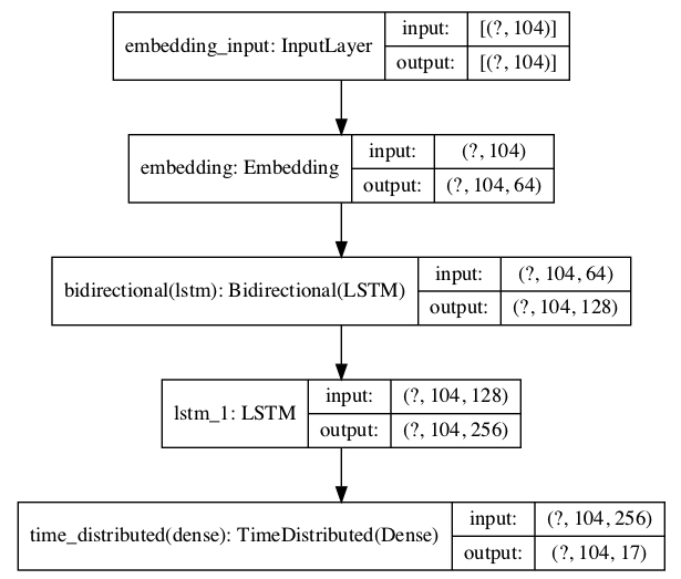
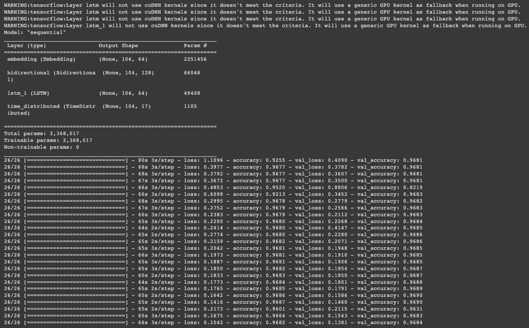
The neural network models uses a graphical structure. As a result, we'll need to first build the architecture and determine the input and output dimensions for each layer. RNNs can handle a wide range of input and output combinations. For this request, we will use a variety of architectures. Take a look at the last architecture in the photograph below. At each time step, we must output a tag (y) for a token (X) ingested.

^source

For reproducibility, it is always suggested to use seed.

seed(1)
tensorflow.random.set_seed(2)

You can also try this code with Online Python Compiler

Run Code

Compare the layers in the model plot with the brief on each layer provided in the image (model-plot) below to gain a better grasp of the layers' input and output dimensions.

To output the result, we are basically working with three layers (embedding, bi-lstm, and lstm layers) and a fourth layer (TimeDistributed Dense layer). In the sections below, we'll go over all the layers.

^source

Layer1

Embedding Layer: The maximum length (104) of the padded sequences will be specified in the embedding layer. After the network has been trained, the embedding layer will convert each token into an n-dimensional vector. We've picked n as the number of dimensions (64).

Layer2

Bidirectional LSTM Layer: A recurrent layer (for example, the first LSTM layer) is passed as an argument to bidirectional LSTM. The output from the preceding embedding layer is used in this layer (104, 64).

Layer3

LSTM Layer: An LSTMnetwork is a type of recurrent neural network that uses LSTM cell blocks instead of traditional neural network layers. The input gate, the forget gate, and the output gate are all components of these cells.

Layer4

Time Distributed Layer: We're working with a Many to Many RNN Architecture, which means we're anticipating output from each input sequence. As an example, in the sequence (a1 b1, a2 b2,...an bn), a and b represent the sequence's inputs and outputs, respectively. Dense(fully-connected) operation across every output over every time step is possible with the TimeDistributeDense layers. If you don't use this layer, you'll only get one final output.

iD = len(list(set(data['Word'].to_list())))+1
oD = 64
iL = max([len(s) for s in dgrp['Word_idx'].tolist()])
n_tags = len(ta2i)
print('input dim: ', iD, '\noutput dim: ', oD, '\ninput length: ', iL, '\nn tags: ', n_tags)

You can also try this code with Online Python Compiler

Run Code

input dim:  35179 
output dim:  64 
input length:  104 
n tags:  17

You can also try this code with Online Python Compiler

Run Code

The code for the model architecture is given below.

def get_bilstm_lstm_model():
   m = Sequential()

   # Adding Embedding layer
   m.add(Embedding(input_dim=iD, output_dim=oD, input_length=iL))

   # Adding bidirectional LSTM
   m.add(Bidirectional(LSTM(units=oD, return_sequences=True, dropout=0.2, recurrent_dropout=0.2), merge_mode = 'concat'))

   # Adding LSTM
   m.add(LSTM(units=oD, return_sequences=True, dropout=0.5, recurrent_dropout=0.5))

   # Adding timeDistributed Layer
   m.add(TimeDistributed(Dense(n_tags, activation="relu")))

   # Compile model
   m.compile(loss='categorical_crossentropy', optimizer='adam', metrics=['accuracy'])
   m.summary()
  
   return m

You can also try this code with Online Python Compiler

Run Code

Train the model

def train_model(X, y, m):
   l = list()
   for i in range(25):
       # fitting model for one epoch on this sequence
       hist = m.fit(X, y, batch_size=1000, verbose=1, epochs=1, validation_split=0.2)
       l.append(hist.history['loss'][0])
   return l

results = pd.DataFrame()
model_bilstm_lstm = get_bilstm_lstm_model()
results['with_add_lstm'] = train_model(train_tokens, np.array(train_tags), model_bilstm_lstm)

You can also try this code with Online Python Compiler

Run Code

Testing our Model

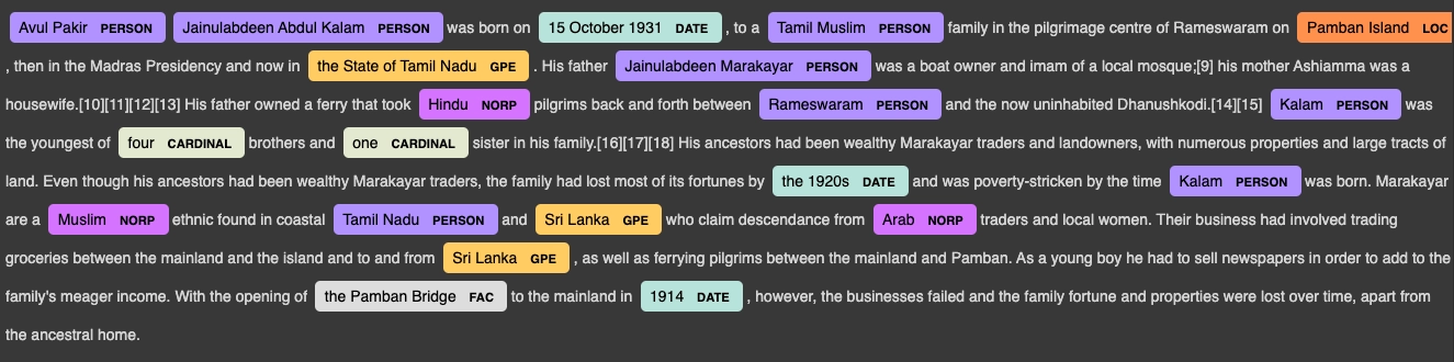
import spacy
from spacy import displacy
nlp = spacy.load('en_core_web_sm')
text = nlp("Avul Pakir Jainulabdeen Abdul Kalam was born on 15 October 1931, to a Tamil Muslim family in the pilgrimage centre of Rameswaram on Pamban Island, then in the Madras Presidency and now in the State of Tamil Nadu. His father Jainulabdeen Marakayar was a boat owner and imam of a local mosque;[9] his mother Ashiamma was a housewife.[10][11][12][13] His father owned a ferry that took Hindu pilgrims back and forth between Rameswaram and the now uninhabited Dhanushkodi.[14][15] Kalam was the youngest of four brothers and one sister in his family.[16][17][18] His ancestors had been wealthy Marakayar traders and landowners, with numerous properties and large tracts of land. Even though his ancestors had been wealthy Marakayar traders, the family had lost most of its fortunes by the 1920s and was poverty-stricken by the time Kalam was born. Marakayar are a Muslim ethnic found in coastal Tamil Nadu and Sri Lanka who claim descendance from Arab traders and local women. Their business had involved trading groceries between the mainland and the island and to and from Sri Lanka, as well as ferrying pilgrims between the mainland and Pamban. As a young boy he had to sell newspapers in order to add to the family's meager income. With the opening of the Pamban Bridge to the mainland in 1914, however, the businesses failed and the family fortune and properties were lost over time, apart from the ancestral home.")
displacy.render(text, style = 'ent', jupyter=True)

You can also try this code with Online Python Compiler

Run Code

You can take any text for testing our model. I have taken the above paragraph from here.

FAQs

1. What is the NER model?

Natural Language Processing (NLP) application named entity recognition (NER) processes and recognizes vast amounts of unstructured human language. Entity identification, entity chunking, and entity extraction are other terms for the same thing.

2. How does NER work with NLP?

The semantic element of NLP, which extracts the meaning of words, sentences, and their relationships, relies heavily on NER. Basic NER identifies and locates entities in structured and unstructured texts.

3. How does spaCy's NER work?

NER locates and categorizes identified entities included in unstructured text into standard categories such as person names, locations, organizations, time expressions, amounts, monetary values, percentages, codes, and so on.