Do you think IIT Guwahati certified course can help you in your career?
Introduction
Machine learning is a sub-field of Artificial Intelligence that is changing the world. It affects almost every aspect of our life. Machine learning algorithms differ from traditional algorithms because no human interaction is needed to improve the model. It learns from data and improves accordingly. There are many algorithms used to make this self-learning possible. We will explore one of the algorithms called Nesterov Accelerated Gradient (NAG)
What is an Optimizer?
An optimizer is an algorithm used in machine learning and deep learning to minimize the loss function by adjusting the model’s parameters (weights and biases). It improves model accuracy by finding the optimal set of parameters that reduce prediction errors.
Gradient descent
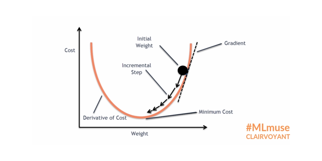
It is essential to understand Gradient descent before we look at Nesterov Accelerated Algorithm. Gradient descent is an optimization algorithm that is used to train our model. The accuracy of a machine learning model is determined by the cost function. The lower the cost, the better our machine learning model is performing. Optimization algorithms are used to reach the minimum point of our cost function. Gradient descent is the most common optimization algorithm. It takes parameters at the start and then changes them iteratively to reach the minimum point of our cost function.
As we can see above, we take some initial weight, and according to that, we are positioned at some point on our cost function. Now, gradient descent tweaks the weight in each iteration, and we move towards the minimum of our cost function accordingly.
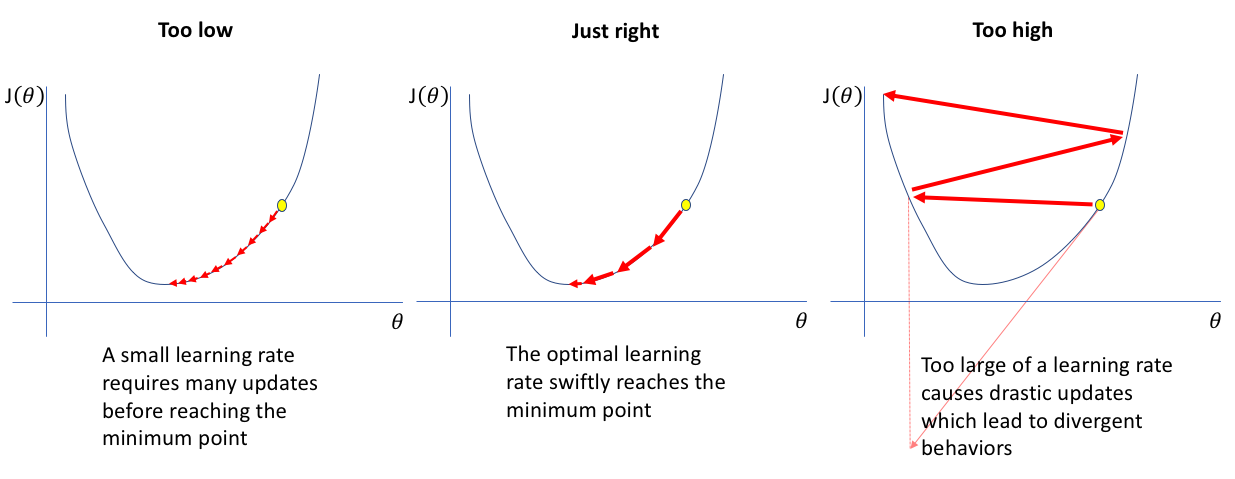
The size of our steps depends onthe learning rate of our model. The higher the learning rate, the higher the step size. Choosing the correct learning rate for our model is very important as it can cause problems while training.
A low learning rate assures us to reach the minimum point, but it takes a lot of iterations to train, while a very high learning rate can cause us to cross the minimum point, a problem commonly known as overshooting.
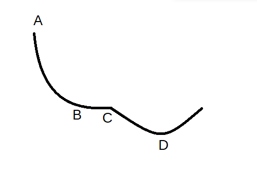
The main drawback of gradient descent is that it depends on the learning rate and the gradient of that particular step only. The gradient at the plateau, also known as saddle points of our function, will be close to zero. The step size becomes very small or even zero. Thus, the update of our parameters is very slow at a gentle slope.
Let us look at an example. The starting point of our model is ‘A’. The loss function will decrease rapidly on the path AB because of the higher gradient. But as the gradient decreases from B to C, the learning is negligible. The gradient at point ‘C’ is zero, and it is the saddle point of our function. Even after many iterations, we will be stuck at ‘C’ and will not reach the desired minimum ‘D’.
This problem is solved by using momentum in our gradient descent.
Gradient descent with momentum
The issue discussed above can be solved by including the previous gradients in our calculation. The intuition behind this is if we are repeatedly asked to go in a particular direction, we can take bigger steps towards that direction.
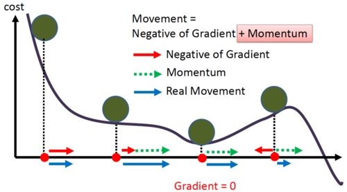
The weighted average of all the previous gradients is added to our equation, and it acts as momentum to our step.
We can understand gradient descent with momentum from the above image. As we start to descend, the momentum increases, and even at gentle slopes where the gradient is minimal, the actual movement is large due to the added momentum.
But this added momentum causes a different type of problem. We actually cross the minimum point and have to take a U-turn to get to the minimum point. Momentum-based gradient descent oscillates around the minimum point, and we have to take a lot of U-turns to reach the desired point. Despite these oscillations, momentum-based gradient descent is faster than conventional gradient descent.
To reduce these oscillations, we can use Nesterov Accelerated Gradient.
Nesterov Accelerated Gradient (NAG)
NAG resolves this problem by adding a look ahead term in our equation. The intuition behind NAG can be summarized as ‘look before you leap’. Let us try to understand this through an example.
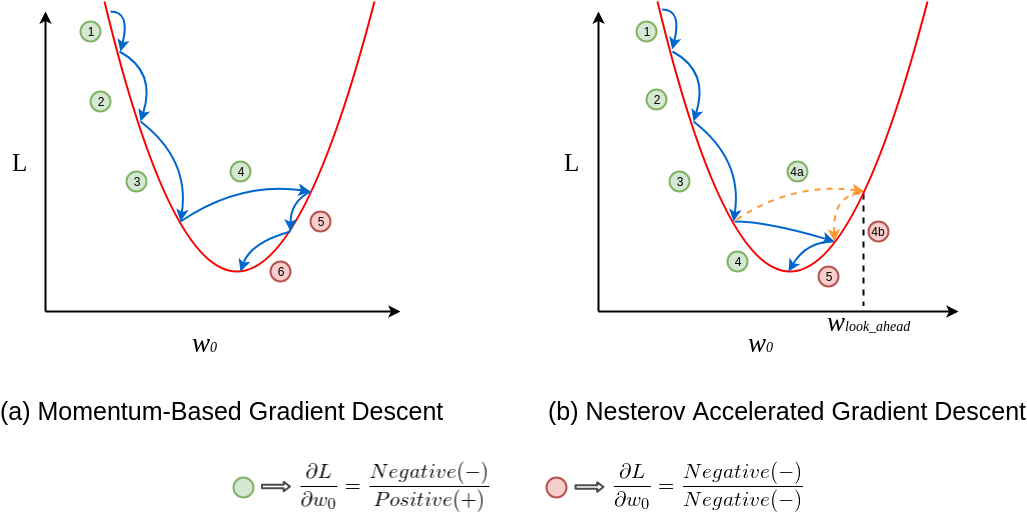
As can see, in the momentum-based gradient, the steps become larger and larger due to the accumulated momentum, and then we overshoot at the 4th step. We then have to take steps in the opposite direction to reach the minimum point.
However, the update in NAG happens in two steps. First, a partial step to reach the look-ahead point, and then the final update. We calculate the gradient at the look-ahead point and then use it to calculate the final update. If the gradient at the look-ahead point is negative, our final update will be smaller than that of a regular momentum-based gradient. Like in the above example, the updates of NAG are similar to that of the momentum-based gradient for the first three steps because the gradient at that point and the look-ahead point are positive. But at step 4, the gradient of the look-ahead point is negative.
In NAG, the first partial update 4a will be used to go to the look-ahead point and then the gradient will be calculated at that point without updating the parameters. Since the gradient at step 4b is negative, the overall update will be smaller than the momentum-based gradient descent.
We can see in the above example that the momentum-based gradient descent takes six steps to reach the minimum point, while NAG takes only five steps.
This looking ahead helps NAG to converge to the minimum points in fewer steps and reduce the chances of overshooting.
How NAG actually works?
We saw how NAG solves the problem of overshooting by ‘looking ahead’. Let us see how this is calculated and the actual math behind it.
Update rule for gradient descent: wt+1 = wt − η∇wt In this equation, the weight (W) is updated in each iteration. η is the learning rate, and ∇wt is the gradient.
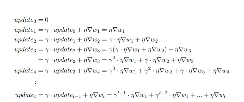
Update rule for momentum-based gradient descent: In this, momentum is added to the conventional gradient descent equation. The update equation is wt+1 = wt − updatet
This is how the gradient of all the previous updates is added to the current update.
Update rule for NAG: wt+1 = wt − updatet While calculating the updatet, We will include the look ahead gradient (∇wlook_ahead). updatet = γ · updatet−1 + η∇wlook_ahead
This look-ahead gradient will be used in our update and will prevent overshooting.
Advantages of Nesterov Accelerated Gradient (NAG):
Faster Convergence – NAG anticipates the future position and adjusts gradients accordingly, leading to quicker optimization.
Reduced Oscillations – Unlike standard momentum, it smooths out updates, preventing overshooting and unnecessary fluctuations.
Improved Stability – Works well with non-convex functions, helping deep learning models train more efficiently.
Better Directional Control – By computing gradients at the lookahead position, NAG provides more accurate updates.
Widely Used in Deep Learning – Incorporated in optimizers like SGD with momentum, improving training speed in frameworks like TensorFlow and PyTorch.
Frequently Asked Questions
What is NAG in deep learning?
Nesterov Accelerated Gradient (NAG) is an optimization technique that improves gradient descent by applying momentum with a lookahead step to achieve faster and smoother convergence.
What is Nesterov in SGD?
Nesterov in Stochastic Gradient Descent (SGD) modifies momentum-based updates by computing the gradient at a future position, improving accuracy and reducing oscillations in optimization.
What is the difference between momentum with GD and Nesterov Accelerated GD?
Momentum-based GD updates using the previous velocity, whereas Nesterov Accelerated GD first moves in the momentum direction, then adjusts using the gradient at the lookahead position.
Conclusion
We started this article by looking at Gradient descent and how it is used to reach the minimum point of our cost function. We also saw its drawback and how it is mitigated by using momentum. Finally, we talked about the Nesterov Accelerated Gradient and how it improves the gradient descent with momentum. We also looked at the in-depth functioning of these algorithms. To dive deeper into the realm of Machine learning, check out our machine learning course at coding ninjas.


 9+ registered

