Table of contents
1.
Introduction
2.
Nonhomogeneous Differential Equations Definition
3.
How To Solve Nonhomogeneous Differential Equations?
4.
How To Find Particular Solution of a Nonhomogeneous Differential Equation?
4.1.
Method of Undetermined Coefficients
4.2.
Method of Variation of Parameters
5.
FAQs
6.
Key Takeaways
Last Updated: Mar 27, 2024

Nonhomogeneous Differential Equations

Author Rajat Agrawal
1 upvote
Career growth poll
Do you think IIT Guwahati certified course can help you in your career?

Introduction

Nonhomogeneous differential equations are the differential equations that contain functions on the right-hand side of the equations. Nonhomogeneous linear equations have many applications in day-to-day life. Laws of motion, for example,  rely on nonhomogeneous differential equations.

Let’s learn about nonhomogeneous differential equations and how to solve them in-depth.

Nonhomogeneous Differential Equations Definition

Nonhomogeneous differential equations are the differential equations that contain functions on the right-hand side of the equations. 

We know that homogeneous differential equations are those equations having zero at R.H.S of the equation.

Examples of homogeneous and non-homogeneous differential equations are shown below. We'll learn how to recognize differential equations based on their form using these examples.

Since we've been working with non-homogeneous linear differential equations of first and second order, here are their general forms:

First-Order: <math xmlns="http://www.w3.org/1998/Math/MathML"><mstyle mathsize="20px"><msup><mi>y</mi><mo>'</mo></msup><mo>+</mo><mi>P</mi><mfenced><mi>x</mi></mfenced><mi>y</mi><mo>&#xA0;</mo><mo>=</mo><mo>&#xA0;</mo><mi>f</mi><mfenced><mi>x</mi></mfenced></mstyle></math>

Second-Order: <math xmlns="http://www.w3.org/1998/Math/MathML"><mstyle mathsize="20px"><msup><mi>y</mi><mrow><mo>'</mo><mo>'</mo></mrow></msup><mo>+</mo><mi>P</mi><mfenced><mi>x</mi></mfenced><msup><mi>y</mi><mo>'</mo></msup><mo>+</mo><mi>Q</mi><mfenced><mi>x</mi></mfenced><mi>y</mi><mo>&#xA0;</mo><mo>=</mo><mo>&#xA0;</mo><mi>g</mi><mfenced><mi>x</mi></mfenced></mstyle></math>

In the next section, we’ll learn how to solve these equations.

How To Solve Nonhomogeneous Differential Equations?

Non-homogeneous linear differential equations can be solved by obtaining the general solution of the corresponding homogeneous differential equation, <math xmlns="http://www.w3.org/1998/Math/MathML"><msub><mi>y</mi><mi>h</mi></msub></math>, and the particular solution of the non-homogeneous equation, <math xmlns="http://www.w3.org/1998/Math/MathML"><msub><mi>y</mi><mi>p</mi></msub></math>.

Particular Solution: A solution yP(x) of a differential equation that contains no arbitrary constants is known as a particular solution to the equation.

Assume we have a non-homogeneous linear differential equation of second order, as given below.

<math xmlns="http://www.w3.org/1998/Math/MathML"><mstyle mathsize="20px"><msup><mi>y</mi><mrow><mo>'</mo><mo>'</mo></mrow></msup><mo>+</mo><mi>a</mi><msup><mi>y</mi><mo>'</mo></msup><mo>+</mo><mi>b</mi><mi>y</mi><mo>&#xA0;</mo><mo>=</mo><mo>&#xA0;</mo><mi>g</mi><mfenced><mi>x</mi></mfenced></mstyle></math>

<math xmlns="http://www.w3.org/1998/Math/MathML"><mi>y</mi><mo>'</mo><mo>'</mo><mo>+</mo><mi>a</mi><mi>y</mi><mo>'</mo><mo>+</mo><mi>b</mi><mi>y</mi><mo>&#xA0;</mo><mo>=</mo><mo>&#xA0;</mo><mn>0</mn></math> is known as the complementary equation.

Both a and b are constants in this equation. As a result, the nonhomogeneous differential equation with a general solution arises, as shown below.

<math xmlns="http://www.w3.org/1998/Math/MathML"><mstyle mathsize="20px"><mi>y</mi><mo>&#xA0;</mo><mo>=</mo><mo>&#xA0;</mo><msub><mi>y</mi><mi>h</mi></msub><mo>+</mo><msub><mi>y</mi><mi>p</mi></msub></mstyle></math>

<math xmlns="http://www.w3.org/1998/Math/MathML"><mstyle mathsize="20px"><msub><mi>y</mi><mi>h</mi></msub></mstyle></math>: General Solution

<math xmlns="http://www.w3.org/1998/Math/MathML"><mstyle mathsize="20px"><msub><mi>y</mi><mi>p</mi></msub></mstyle></math>: Particular Solution

The nth-order non-homogeneous linear differential equation can be used to extend this. This linear differential equation's general solution is provided below.

<math xmlns="http://www.w3.org/1998/Math/MathML"><mstyle mathsize="20px"><msub><mi>c</mi><mn>1</mn></msub><msub><mi>y</mi><mn>1</mn></msub><mo>+</mo><msub><mi>c</mi><mn>2</mn></msub></mstyle></math>

How To Find Particular Solution of a Nonhomogeneous Differential Equation?

There are the two most frequent methods for determining the particular solution of a non-homogeneous differential equation:

1.) Method of Undetermined Coefficients

2.) Method of Variation of Parameters

Method of Undetermined Coefficients

Let's break down the steps of the method of undetermined coefficients and identify when it's appropriate to utilize it. When the right-hand side of our non-homogeneous differential equation is a function that can be expressed as the sum or product of the following functions, the undetermined coefficient technique works best: <math xmlns="http://www.w3.org/1998/Math/MathML"><msup><mi>e</mi><mi>x</mi></msup><mo>,</mo><mo>&#xA0;</mo><msup><mi>x</mi><mi>n</mi></msup><mo>,</mo><mo>&#xA0;</mo><mi>cos</mi><mfenced><mrow><mi>&#x3B2;</mi><mi>x</mi></mrow></mfenced><mo>&#xA0;</mo><mi>o</mi><mi>r</mi><mo>&#xA0;</mo><mi>sin</mi><mfenced><mrow><mi>&#x3B2;</mi><mi>x</mi></mrow></mfenced></math>

<math xmlns="http://www.w3.org/1998/Math/MathML"><mi>y</mi><mo>&quot;</mo><mo>+</mo><mi>a</mi><mi>y</mi><mo>'</mo><mo>+</mo><mi>b</mi><mi>y</mi><mo>&#xA0;</mo><mo>=</mo><mo>&#xA0;</mo><mi>g</mi><mfenced><mi>x</mi></mfenced></math>

Once we identify the form of g(x), we guess for the particular solution, yp. We have shown some examples below where we guessed the particular solution for some g(x).

Let’s look at the example below to understand how this method works.

Example: Find the general solution to <math xmlns="http://www.w3.org/1998/Math/MathML"><mi>y</mi><mo>'</mo><mo>'</mo><mo>+</mo><mn>4</mn><mi>y</mi><mo>'</mo><mo>+</mo><mn>3</mn><mi>y</mi><mo>&#xA0;</mo><mo>=</mo><mo>&#xA0;</mo><mn>3</mn><mi>x</mi></math>.

Solution: The complementary equation is <math xmlns="http://www.w3.org/1998/Math/MathML"><mi>y</mi><mo>'</mo><mo>'</mo><mo>+</mo><mn>4</mn><mi>y</mi><mo>'</mo><mo>+</mo><mn>3</mn><mi>y</mi><mo>&#xA0;</mo><mo>=</mo><mo>&#xA0;</mo><mn>0</mn></math>, with the general solution <math xmlns="http://www.w3.org/1998/Math/MathML"><msub><mi>c</mi><mn>1</mn></msub><msup><mi>e</mi><mrow><mo>-</mo><mi>x</mi></mrow></msup><mo>+</mo><msub><mi>c</mi><mn>2</mn></msub><msup><mi>e</mi><mrow><mo>-</mo><mn>3</mn><mi>x</mi></mrow></msup></math>

Since, r(x) = 3x, the particular equation might have form <math xmlns="http://www.w3.org/1998/Math/MathML"><msub><mi>y</mi><mi>p</mi></msub><mfenced><mi>x</mi></mfenced><mo>&#xA0;</mo><mo>=</mo><mo>&#xA0;</mo><mi>a</mi><mi>x</mi><mo>+</mo><mi>b</mi></math>. In this case 

<math xmlns="http://www.w3.org/1998/Math/MathML"><msub><mi>y</mi><mi>p</mi></msub><mo>'</mo><mo>&#xA0;</mo><mfenced><mi>x</mi></mfenced><mo>=</mo><mo>&#xA0;</mo><mi>a</mi><mo>&#xA0;</mo><mi>a</mi><mi>n</mi><mi>d</mi><mo>&#xA0;</mo><msub><mi>y</mi><mi>p</mi></msub><mo>'</mo><mo>'</mo><mfenced><mi>x</mi></mfenced><mo>&#xA0;</mo><mo>=</mo><mo>&#xA0;</mo><mn>0</mn></math>  For  𝑦𝑝  to be a solution to the differential equation, we must find values for a  and  b  such that

<math xmlns="http://www.w3.org/1998/Math/MathML"><mi>y</mi><mo>'</mo><mo>'</mo><mo>+</mo><mn>4</mn><mi>y</mi><mo>'</mo><mo>+</mo><mn>3</mn><mi>y</mi><mo>&#xA0;</mo><mo>=</mo><mo>&#xA0;</mo><mn>3</mn><mi>x</mi><mspace linebreak="newline"/><mn>0</mn><mo>+</mo><mn>4</mn><mfenced><mi>a</mi></mfenced><mo>+</mo><mn>3</mn><mfenced><mrow><mi>a</mi><mi>x</mi><mo>+</mo><mi>b</mi></mrow></mfenced><mo>&#xA0;</mo><mo>=</mo><mo>&#xA0;</mo><mn>3</mn><mi>x</mi><mspace linebreak="newline"/><mn>3</mn><mi>a</mi><mi>x</mi><mo>+</mo><mfenced><mrow><mn>4</mn><mi>a</mi><mo>+</mo><mn>3</mn><mi>b</mi></mrow></mfenced><mo>&#xA0;</mo><mo>=</mo><mo>&#xA0;</mo><mn>3</mn><mi>x</mi></math>

Equalizing the coefficients, we get:

3a = 3 => a = 1

4a+3b = 0 => b = -4/3

Therefore, <math xmlns="http://www.w3.org/1998/Math/MathML"><msub><mi>y</mi><mi>p</mi></msub><mfenced><mi>x</mi></mfenced><mo>&#xA0;</mo><mo>=</mo><mo>&#xA0;</mo><mi>x</mi><mo>&#xA0;</mo><mo>-</mo><mfrac><mrow><mo>&#xA0;</mo><mn>4</mn></mrow><mn>3</mn></mfrac></math> and the general solution is <math xmlns="http://www.w3.org/1998/Math/MathML"><mi>y</mi><mfenced><mi>x</mi></mfenced><mo>&#xA0;</mo><mo>=</mo><mo>&#xA0;</mo><msub><mi>c</mi><mn>1</mn></msub><msup><mi>e</mi><mrow><mo>-</mo><mi>x</mi></mrow></msup><mo>+</mo><msub><mi>c</mi><mn>2</mn></msub><msup><mi>e</mi><mrow><mo>-</mo><mn>3</mn><mi>x</mi></mrow></msup><mo>+</mo><mi>x</mi><mo>-</mo><mfrac><mn>4</mn><mn>3</mn></mfrac></math>.

Method of Variation of Parameters

r(x) isn't always made up of polynomials, exponentials, or sines and cosines. When this happens, the method of undetermined coefficients fails, and we must apply an alternative method to obtain a specific solution to the differential equation. We use a technique known as the method of Variation of parameters.

Let's say we have a non-homogeneous linear differential equation of second order, as given below.

<math xmlns="http://www.w3.org/1998/Math/MathML"><mi>y</mi><mo>'</mo><mo>'</mo><mo>+</mo><mi>p</mi><mi>y</mi><mo>'</mo><mo>+</mo><mi>q</mi><mi>y</mi><mo>&#xA0;</mo><mo>=</mo><mo>&#xA0;</mo><mi>r</mi><mfenced><mi>x</mi></mfenced></math>, where p and q are constants.

If the general solution to the complementary equation is given by <math xmlns="http://www.w3.org/1998/Math/MathML"><msub><mi>c</mi><mn>1</mn></msub><msub><mi>y</mi><mn>1</mn></msub><mfenced><mi>x</mi></mfenced><mo>+</mo><msub><mi>c</mi><mn>2</mn></msub><msub><mi>y</mi><mn>2</mn></msub><mfenced><mi>x</mi></mfenced></math>, then the particular solution is given by <math xmlns="http://www.w3.org/1998/Math/MathML"><msub><mi>y</mi><mi>p</mi></msub><mfenced><mi>x</mi></mfenced><mo>&#xA0;</mo><mo>=</mo><mo>&#xA0;</mo><mi>u</mi><mfenced><mi>x</mi></mfenced><msub><mi>y</mi><mn>1</mn></msub><mfenced><mi>x</mi></mfenced><mo>+</mo><mi>v</mi><mfenced><mi>x</mi></mfenced><msub><mi>y</mi><mn>2</mn></msub><mfenced><mi>x</mi></mfenced></math>


Read Also -  Difference between argument and parameter

FAQs

1. Define Nonhomogeneous Differential Equation.

Nonhomogeneous differential equations are the differential equations that contain functions on the right-hand side of the equations. 

2. Mention some examples of the Nonhomogeneous differential equations. 

A few examples of Nonhomogeneous differential equations are:-

a.) y’’+y’-5y = sin(x)

b.) y’’-10y’+6y = 4x+5

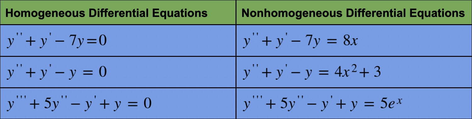
3. What is the difference between homogeneous and nonhomogeneous differential equations?

In homogeneous differential equation, the equation has zero in R.H.S while in nonhomogeneous differential equation, it contains functions on the right-hand side of the equation.

Key Takeaways

In this article, we have extensively discussed Nonhomogeneous Differential Equations, their definition, and how to solve nonhomogeneous differential equations. If you want to learn more, check out our articles on the Partial Differential Equations, and System of Linear Equations.

Do upvote our blog to help other ninjas grow.

Happy Coding!

Live masterclass