


Introduction
The Normal Distribution is also known as the Gaussian Distribution and Bell-Shaped Distribution. When a random experiment is replicated, the random variable that will equal the average or total result over the replicates will have a normal distribution as the number of replicates becomes large.
Probability Density Function
For −∞<μ<∞ and σ>0, the Normal Distribution is denoted by N(μ,σ2), and its probability density is given by
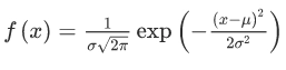 .
.
σ is the Standard Deviation, and μ is the Mean.
Let’s break the formula into smaller pieces to understand what’s happening.
Z-score - It measures how many standard deviations away a data point lies from the mean.
 .
.
The exp in the above probability density formula is the square of the z-score times -½. The values that are away from the mean have a lower probability than those near the mean. The values away from the mean have a higher z-score and thus a lower probability since the exp is negative. The vice-versa is for the values closer to the mean.
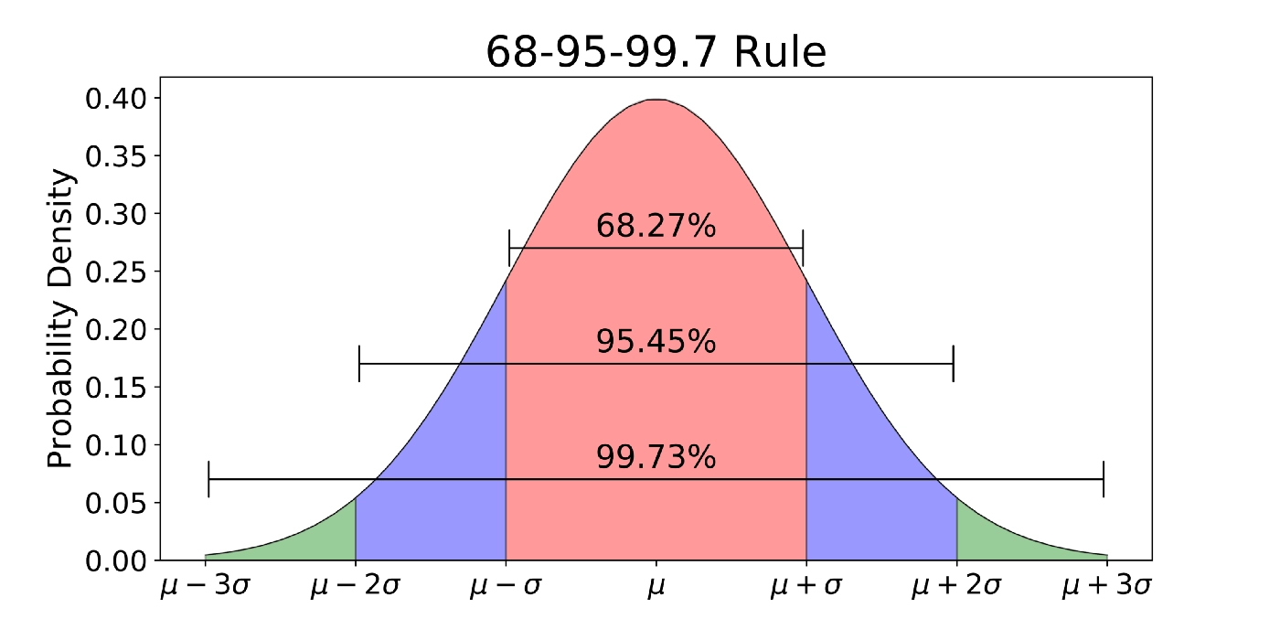
Now comes the 68-95-99.7 rule. The rule states that the % of values within a band around the mean in a normal distribution having a width of two, four, and six standard deviations comprise 68%, 95%, and 99.7% of all the values.
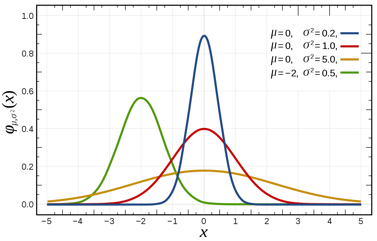
The effects of σ and μ on the Distribution are shown in the above picture.
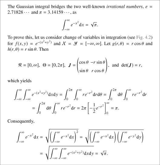
The above f(x) is integrated into one, which can be proved by the Gaussian integral below.
Let ‘X’ = normal distributed random variable with parameters μ and σ^2. The area inside the normal distribution curve is 1 as the probability is 1.
Thus,  = 1;
= 1;

writing x as (x-μ ) + μ yields

Letting y=x-μ

The first part is symmetric about the y-axis, hence its value is 0.


Thus,
Expectation E[x] = μ
Variance = σ^2
Standard Deviation =  .
.


 9+ registered

