Implementation
You can download the dataset from here. Video link can be found here.
import cv2
import numpy as np
import math
import copy
def jacobian(x_shape, y_shape):
# get jacobian of the template size.
x = np.array(range(x_shape))
y = np.array(range(y_shape))
x, y = np.meshgrid(x, y)
ones = np.ones((y_shape, x_shape))
zeros = np.zeros((y_shape, x_shape))
row1 = np.stack((x, zeros, y, zeros, ones, zeros), axis=2)
row2 = np.stack((zeros, x, zeros, y, zeros, ones), axis=2)
jacob = np.stack((row1, row2), axis=2)
return jacob
def get_template(image, roi, num_layers):
template = cv2.cvtColor(image, cv2.COLOR_BGR2GRAY)
template = cv2.GaussianBlur(template, (5, 5), 5)
template = resample_image(template, num_layers, resample=cv2.pyrDown)
scale_down = 1/2**num_layers
roi = (roi * scale_down).astype(int)
#template = (template - np.mean(template)) / np.std(template)
#return crop(template, roi)
return template
def normalize_image(image, template):
image = (image * (np.mean(template)/np.mean(image))).astype(float)
return image
def resample_image(image, iteration, resample):
for i in range(iteration):
image = resample(image)
return image
def crop(img, roi):
return img[roi[0][1]:roi[1][1], roi[0][0]:roi[1][0]]
def gamma_correction(image, gamma=1.0):
# build a lookup table mapping the pixel values [0, 255] to
# their adjusted gamma values
invGamma = 1.0 / gamma
table = np.array([((i / 255.0) ** invGamma) * 255
for i in np.arange(0, 256)]).astype("uint8")
# apply gamma correction using the lookup table
return cv2.LUT(image, table)
def equalize_light(image, limit=12.0, grid=(2,2), gray=False):
if (len(image.shape) == 2):
image = cv2.cvtColor(image, cv2.COLOR_GRAY2BGR)
gray = True
clahe = cv2.createCLAHE(clipLimit=limit, tileGridSize=grid)
lab = cv2.cvtColor(image, cv2.COLOR_BGR2LAB)
l, a, b = cv2.split(lab)
cl = clahe.apply(l)
#cl = cv2.equalizeHist(l)
limg = cv2.merge((cl,a,b))
image = cv2.cvtColor(limg, cv2.COLOR_LAB2BGR)
if gray:
image = cv2.cvtColor(image, cv2.COLOR_BGR2GRAY)
return np.uint8(image)
def update_roi_bolt(frame, roi):
roi_map = {
50: np.array([[221, 73], [278, 173]]),
110: np.array([[206, 53], [269, 174]]),
150: np.array([[272, 70], [319, 166]]),
190: np.array([[327, 66], [381, 162]]),
220: np.array([[327, 89], [382, 172]]),
250: np.array([[351, 98], [420, 173]]),
280: np.array([[351, 85], [410, 176]]),
}
return roi_map.get(frame, roi)
def update_roi_car(frame, roi):
roi_map = {
50: np.array([[64, 52], [167, 133]]),
100: np.array([[81, 58], [163, 127]]),
130: np.array([[82, 64], [176, 138]]),
160: np.array([[100, 55], [199, 134]]),
180: np.array([[116, 59], [198, 128]]),
210: np.array([[135, 60], [227, 130]]),
240: np.array([[160, 58], [248, 126]]),
280: np.array([[191, 59], [261, 119]]),
320: np.array([[200, 65], [278, 122]]),
400: np.array([[221, 74], [295, 128]])
}
return roi_map.get(frame, roi)
def update_roi_baby(frame, roi):
roi_map = {
14: np.array([[133, 78], [207, 141]]),
44: np.array([[21, 44], [135, 105]]),
55: np.array([[193, 81], [259, 132]]),
80: np.array([[94, 133], [209, 252]]),
90: np.array([[166, 63], [253, 160]])
}
return roi_map.get(frame, roi)
def affineLKtracker(img, template, rect, p, threshold, check_brightness, max_iter=100):
d_p_norm = np.inf
template = crop(template, rect)
rows, cols = template.shape
#img = (img-np.mean(img))/np.std(img)
p_prev = p
iter = 0
while (d_p_norm >= threshold) and iter <= max_iter:
warp_mat = np.array([[1+p_prev[0], p_prev[2], p_prev[4]], [p_prev[1], 1+p_prev[3], p_prev[5]]])
warp_img = crop(cv2.warpAffine(img, warp_mat, (img.shape[1],img.shape[0]),flags=cv2.INTER_CUBIC), rect)
if check_brightness and np.linalg.norm(warp_img) < np.linalg.norm(template):
#warp_img = gamma_correction(warp_img.astype(int), gamma=1.5)
print('inside')
warp_img = equalize_light(warp_img.astype(int))
diff = template.astype(int) - warp_img.astype(int)
# Calculate warp gradient of image
grad_x = cv2.Sobel(img, cv2.CV_64F, 1, 0, ksize=5)
grad_y = cv2.Sobel(img, cv2.CV_64F, 0, 1, ksize=5)
#warp the gradient
grad_x_warp = crop(cv2.warpAffine(grad_x, warp_mat, (img.shape[1],img.shape[0]),flags=cv2.INTER_CUBIC+cv2.WARP_INVERSE_MAP), rect)
grad_y_warp = crop(cv2.warpAffine(grad_y, warp_mat, (img.shape[1],img.shape[0]),flags=cv2.INTER_CUBIC+cv2.WARP_INVERSE_MAP), rect)
# Calculate Jacobian for the
jacob = jacobian(cols, rows)
grad = np.stack((grad_x_warp, grad_y_warp), axis=2)
grad = np.expand_dims((grad), axis=2)
#calculate steepest descent
steepest_descents = np.matmul(grad, jacob)
steepest_descents_trans = np.transpose(steepest_descents, (0, 1, 3, 2))
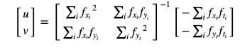
# Compute Hessian matrix
hessian_matrix = np.matmul(steepest_descents_trans, steepest_descents).sum((0,1))
# Compute steepest-gradient-descent update
diff = diff.reshape((rows, cols, 1, 1))
update = (steepest_descents_trans * diff).sum((0,1))
# calculate dp and update it
d_p = np.matmul(np.linalg.pinv(hessian_matrix), update).reshape((-1))
p_prev += d_p
d_p_norm = np.linalg.norm(d_p)
iter += 1
return p_prev
def pyr_LK_Tracker(image, template, roi, num_layers, threshold, check_brightness):
image_copy = copy.deepcopy(image)
template_copy = copy.deepcopy(template)
scale_down = 1/2**num_layers
scale_up = 2**num_layers
roi_down = (roi*scale_down).astype(int)
image = resample_image(image, num_layers, resample=cv2.pyrDown)
p = np.zeros(6)
roi_pyr = roi_down
#num_layers = 0 # to be removed
for i in range(num_layers+1):
p = affineLKtracker(image, template_copy, roi_pyr, p, threshold, check_brightness)
image = resample_image(image, iteration=1, resample=cv2.pyrUp)
template_copy = resample_image(template_copy, iteration=1, resample=cv2.pyrUp)
roi_pyr = (roi_pyr * 2).astype(int)
return p
if __name__ == "__main__":
frame = 1
frame_str = str(frame).zfill(4)
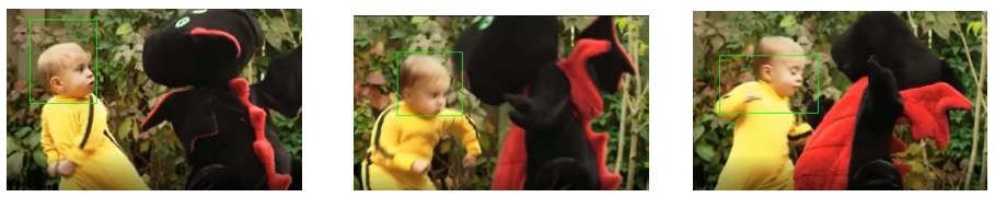
folder_path = 'DragonBaby/img/'
img_file = folder_path + frame_str + '.jpg'
template = cv2.imread(img_file)
height, width, _ = template.shape
#template = cv2.cvtColor(template, cv2.COLOR_BGR2GRAY)
roi = np.array([[149, 63], [223, 154]]) # baby
rect_tl_pt = np.array([roi[0][0], roi[0][1], 1])
rect_br_pt = np.array([roi[1][0], roi[1][1], 1])
frame = 2
fourcc = cv2.VideoWriter_fourcc(*'XVID')
out = cv2.VideoWriter("track_baby3.avi", fourcc, 10.0, (width,height))
num_layers = 1
template_copy = copy.deepcopy(template)
template = get_template(template, roi, num_layers)
threshold = 0.001
while True:
img_file = folder_path + frame_str + '.jpg'
image = cv2.imread(img_file)
if image is None or cv2.waitKey(1) == 27:
print('No Image found')
break
image_copy = copy.deepcopy(image)
image = cv2.cvtColor(image, cv2.COLOR_BGR2GRAY)
image = cv2.GaussianBlur(image, (5, 5), 5)
image = normalize_image(image, template)
p = np.zeros(6)
p_prev = p
p = pyr_LK_Tracker(image, template, roi, num_layers, threshold, False)
warp_mat = np.array([[1 + p[0], p[2], p[4]], [p[1], 1 + p[3], p[5]]])
rect_tl_pt_new = (warp_mat @ rect_tl_pt).astype(int)
rect_br_pt_new = (warp_mat @ rect_br_pt).astype(int)
cv2.rectangle(image_copy, tuple(rect_tl_pt_new), tuple(rect_br_pt_new), (255, 255, 0), 1)
cv2.imshow('Tracked Image', image_copy)
frame += 1
frame_str = str(frame).zfill(4)
p_prev = p
roi = update_roi_baby(frame, roi)
rect_tl_pt = np.array([roi[0][0], roi[0][1], 1])
rect_br_pt = np.array([roi[1][0], roi[1][1], 1])
#print('frame----------------', frame)
out.write(image_copy)
out.release()
cv2.destroyAllWindows()

You can also try this code with Online Python Compiler
Output:
Applications
Optical flow finds various uses in the domain of deep learning as well as outside of it. Some examples of Optical flow uses outside of deep learning are:
- 3D shape generation from motion
- Global motion compensation used in video compression, and stabilisation.
- Used in autonomous vehicle navigation.
- Used in film industry for intense VFX shots.
Examples of Optical flow applications in the domain of deep learning include:
- Used in smoothening of generative adversarial networks so that outputs can be temporally coherent. This would be a tough task if we were to use only GANs which are unable to encode a temporal coherent.
-
Video recognition using the two-stream architecture where the first stream takes the raw image and the second stream takes a series of optical flow images.
Also read, Sampling and Quantization
FAQs
-
What are the 2 main assumptions of optical flow?
Optical flow assumes that the pixel intensity remains constant across all the frames in a video. The second assumption in optical flow is that the neighbouring pixels are in a similar motion.
-
Mention one limitation of optical flow in digital video processing.
The main problem with the optical flow is that the smoothness of the motion doesn’t allow for discontinuities of motion across object boundaries in a given scene.
Key Takeaways
The blog gives a brief introduction to optical flow and discusses its various applications in deep learning. The blog also gives an implementation of sparse optical flow using Lucas Kannade method. Readers are strongly advised to go through the blog at least a few couple times. If you wish to take a stride forward in your machine learning career, you may want to check out our industry-oriented machine learning courses.


 8+ registered

