Do you think IIT Guwahati certified course can help you in your career?
Introduction
Outliers are data points that deviate significantly from the overall pattern of a dataset. They can arise due to variability in measurement, errors, or rare occurrences and may affect the accuracy of statistical analyses and machine learning models.
In this article, we will learn what outliers are, why they matter, and various techniques to detect them effectively to ensure clean and reliable data for analysis.
What are Outliers?
Outliers are extreme data points in a data set that can be negative or positive, from most of the observations plotted, creating distinctive points in the dataset. Outliers can be informative and valuable in some cases. At the same time, they can even point at insufficient data that creates errors and increase the complexity of the statistical calculations to display the model’s accuracy.
Let's understand outliers with a simple example.
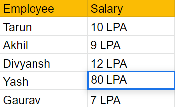
In the case below, Yash's income is the highest relative to the other employees, inflating the group's mean salary and producing inaccurate results. We can see that Yash is the group's outlier and is producing unneeded computation errors in this group. Thus, we exclude Yash and focus on the remaining four employees whose salaries are similar.
Note*: LPA(Lakhs per annum)
But, in real life, the data that one deals with is huge, around 100+ rows and columns that cannot be dealt with manually. Thus we use modern-day techniques to generate accurate results, as per our ML model.
Why do Outliers Exist?
Several factors lead to the occurrence of outliers in a given data set. In this section, we will talk about the most common reasons that lead to outliers in our data that are not particularly needed.
Manual Errors
It is one of the most common types of error seen in large data sets as the data fed to the system is vast and such data entered manually is susceptible to frequent manual errors.
Experimental Errors
Such errors are prominent in the extraction, application, and final implementation of the data set when the initial layout of the model is not structured orderly.
Variability in Data
Data can be of various types and multidimensional, which can cause the data set to contain errors while training the model.
Types of Outliers
Outliers can be briefly classified into three types as mentioned below, depending on the nature of the outlier.
Univariate Outliers
The data points plotted in a given dataset that is too far away from the majority of the data points can be classified as univariate outliers. Univariate outliers can easily be detected visually by plotting the data points of the dataset. Z-score is the best technique to find and categorise univariate outlines when the given data is continuous with standardised values.
Multivariate Outliers
Multivariate outliers are multidimensional and can be noticed only when certain constraints are applied to the data set plotted. They appear to be usual data points when plotted without constraints.
Global Outliers
Global outliers can be simply classified as points in a data set that can be acknowledged in case of a significant deviation from the majority of data values given in the dataset.
Contextual Outliers
Contextual outliers may not highly deviate from the rest of the data set and might look like a part of the general range of the data values given. Yet, under given constraints, the values can turn out to be different, be it higher or lower compared to other data values.
Collective Outliers
As the name suggests, the collective outliers point towards the Kaggleoints clustered away from most of the data set. The values that deviate remarkably from the data sets creating a subset of the data points, come under collective outliers.
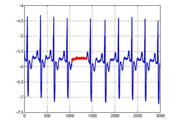
In the above diagram, the part with the red ink refers to the collective outliers.
The part with enormous positive and negative dips is classified as global outliers. But the part with more varied dips than collective outliers but fewer. Dips in the graph than global outliers are classified as a contextual outlier.
Ways to Detect Outliers
Several ways can be used to detect the outliers, including clustering, DBSCAN, isolated forest, hypothesis testing and several others. But, in this section, we will be talking about the most simple techniques to detect outliers in a given dataset.
Using Z-score
Z-score is used to calculate the distance of data points from the calculated mean in the given data set using normal standard deviation. The Z-score is most efficient in dealing with parametric distribution.
By default, the mean of the data is considered to be 0, and the standard deviation is assumed to be 1. Later, we rescale the centre value by derived mean and calculate the standard deviation according to the given data set.
But now the question arises how does z-score work in the case of outliers?
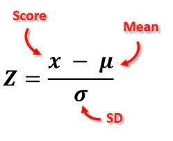
Outliers use the mathematical formula mentioned below.
*Note- As we can see, the z-score is equal to the score or number of observations(x) - the calculated mean(μ), which is divided by the standard deviation(σ).
The next most important thing to know is what range of standard deviation should we take such that the data set points towards the correct sample data, and what is the threshold beyond which the data set points are considered outliers?
The standard threshold value beyond which the data set points are considered to be outliers is +3, -3. That means all the points that lie in the range of the 3rd standard deviation are the correct data points of the dataset and the ones beyond it are outliers.
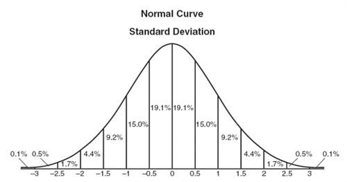
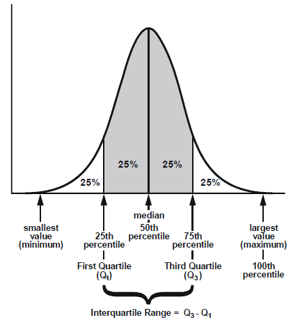
Let’s understand why we take the threshold as 3 from the above bell curve or normal standard deviation curve.
As one can clearly see, from -1 to +1, that is the first standard deviation(σ) from the mean(μ) 0, the percentage of data covered is 68.3%.
Followed by the second deviation(σ), the percentage increases to 95.4%
Followed by the third deviation(σ), we cover about 99.7% of the data points given in our data set.
Thus, we can assume that the rest of the points beyond this range are outliers.
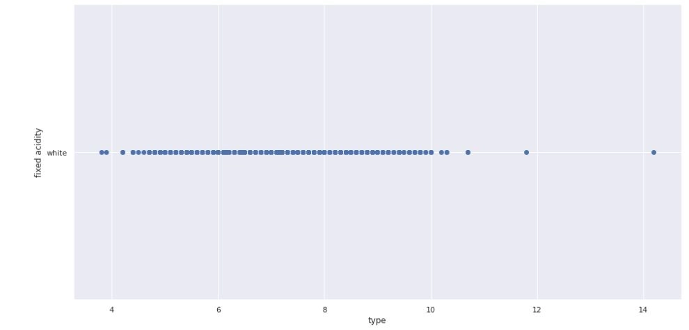
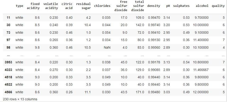
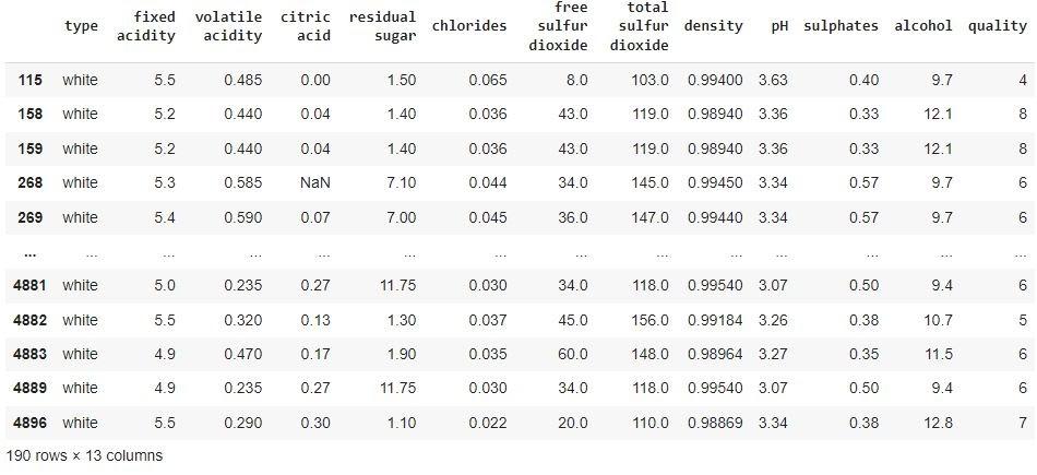
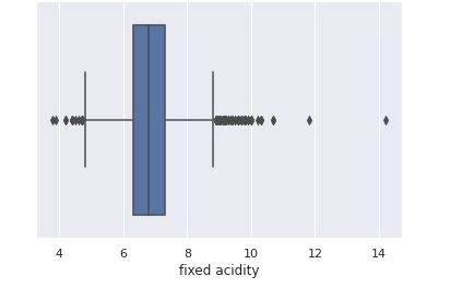
Keeping the above in mind, let’s see how this works, with the “fixed acidity” of the wine from the wine quality dataset imported from Kaggle.
Code
Step 1: First, let’s visualise the dataset better to understand the data under observation, i.e. fixed acidity.
# Let's import the required mathematical libraries
import pandas as pd
import numpy as np
import matplotlib.pyplot as plt
import seaborn as sns; sns.set()

#Import the Dataset
data=pd.read_csv("winequalityN.csv")
data.head()
You can also try this code with Online Python Compiler
#Since we can clearly analyze in the dataset we have outliers lets find them
#z = (X — μ) / σ
fixed_acidity=data["fixed acidity"]
mean_f=np.mean(fixed_acidity)
std_f=np.std(fixed_acidity)
#Create a list for outliers
outliers=[]
threshold=3
for i in fixed_acidity:
    z_score=(i-mean_f)/std_f
#Print Z-score
    if np.abs(z_score)>threshold:
        outliers.append(i)
You can also try this code with Online Python Compiler
As the name suggests, in the percentile technique, we categorise data into the slots of percentile in which most of the data lies from the given data set. This means that given a value from the data sets, we categorise them based on the percentile of the total data they lie in.
Percentiles are very useful for spotting outliers and reflecting a typical experience in data that is expected to vary a lot. Let’s understand how it works.
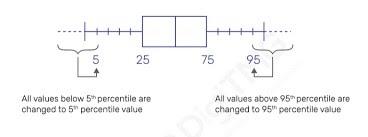
We use relative scores to understand how percentiles work. While using the percentile technique, we focus on data points below or above our calculated percentile threshold of the data set to be 95 percentile for the upper limit and 5 percentile for the lower limit.
We use relative scores to understand how percentiles work. While using the percentile technique, we focus on data points below or above our calculated percentile threshold of the data set to be 95 percentile for the upper limit and 5 percentile for the lower limit.
Outliers are found by setting a threshold that indicates that all the data above 95 percentile of our total data are outliers. All data points below 5 percentile of our total data are considered outliers.
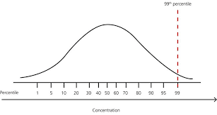
Although for data sets that are well extracted, the ideal percentile values for upper bound are 99 percentile and 1 percentile for the lower bound from which the given data points beyond the range can be considered outliers.
Code
Let’s see this in the form of code and how we can use the above technique to find outliers. In this case, we have taken the upper percentile as 95 and the lower percentile as 5.
Step1: Let’s Define the minimum and maximum threshold value.
Looking at the above output, we can rightly assume that the shown values are all outliers for our data set.
Using InterQuartile range (IQR)
Now that we are familiar with percentiles, let's move on with another technique used to detect outliers using the interquartile technique. We always work on sorted data to avoid mistakes and have an orderly distinction between the data sets while working on IQR.
Once we have the sorted data points, we set our range according to the percentile calculated from the given data set. We categorise them in the following manner.
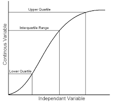
To better understand, the data set can be categorised into 25 percentile known as the first quartile, 50 percentile also known as median, 75 percentile known as the third quartile, and 100 percentile. These slots help us categorise, divide and analyse the variability of the data regarding the data distribution in the given dataset.
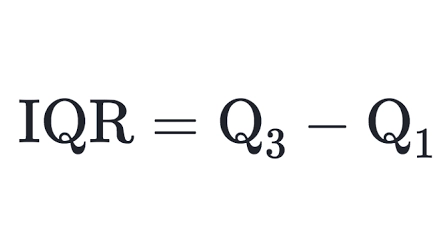
When we talk about the interQuartile range we subtract 75 percentile from the 25 percentile, and whatever the result bears is known as our interQuartile range.
Thus the formulae that we use to calculate the interQuartile range is
Not only do we calculate the percentile, we also calculate the upper and lower bound to categorise the outliers. The upper bound is calculated by Quantile 3 + (1.5 * IQR), and the lower bound is calculated by Quantile 3 - (1.5 * IQR)
We can now acknowledge those values. Beyond the above-stated but, the lower and upper bound values can be categorised as outliers beyond the quartile range.
Z-score Technique
Percentile Technique
IQR Technique
The Z-score technique is best used when the data provided is parametric in nature.
Percentile Technique helps classify large data sets and provide a cumulative result for the dataset.
IQR is best used when the given dataset is skewed in nature.
In large datasets, a z-score might bear incorrect results.
Percentile categorises the data irrespective of their values, making it difficult to analyse the outliers.
The IQR is not amendable by mathematical manipulation.
From the above table, we can positively assume that IQR is the best technique to use as it can work on a bulk of data that can help process and cover outliers from several dimensions in the dataset once you are aware of the IQR.
Several statistical techniques can also be applied to detect outliers, apart from the above-stated method. Hypothesis testing is one of the statistical methods used to calculate outliers from a given data distribution.
Grubbs Test
While using the Grubbs test, we assume our dataset usually is distributed and has two-sided versions where the H0: signifies there are no outliers(Null hypothesis). While the H1: There is at least one outlier. (Alternate hypothesis)
Chi-Square Test
We use chi-square to work out the outlier data points using the logic of frequency compatibility in the given data.
Q-test
The Q-test uses the range and the gap between the data to find the outliers. Although Q-test should only be applied once in the given dataset.
Frequently Asked Questions
When should we remove outliers from the given data sets?
Removing outliers before the transformation of the data set is a better option as it helps create a normal distribution making the data set more effective.
Should we delete all outliers from our data set?
The simple answer is NO! It's essential to classify an outlier before removing it from the data set, as some outliers can help detect informative abnormalities in the recorded data signifying alarming possibilities.
Can we generate outliers in our given data set?
Yes, you can; while creating your random dataset, you can set higher and lower points than the upper and the lower limit.
Conclusion
Outliers can play a crucial role in cases where they can be studied to understand the dataset better. This makes it crucial to understand the type of outlier first to use it for their benefit. In this article, we have discussed the basics of outliers and ways to detect them using techniques such as Z-score, percentile technique, and InterQuartile Range(IQR). To learn better and understand ML concepts in-depth, you can even refer to our blogs on machine learning from our official website.


 18+ registered

