Do you think IIT Guwahati certified course can help you in your career?
What is Principal Component Analysis (PCA)?
Before diving into the technical definition of Principal Component Analysis (PCA), let’s consider a real-world scenario:
Imagine you want to predict real estate prices in a metropolitan city for the year 2021. Several factors influence property prices, including:
Land cost and availability
Price variations by locality
Interest rates and economic indicators (GDP, employment data, inflation, etc.)
Government policies and subsidies
Traffic conditions and infrastructure
Availability of essential facilities (schools, hospitals, public transport, etc.)
Electricity and utility costs
With so many factors in play, analyzing the relationships between all these variables becomes complex. Handling a high number of variables can lead to the following challenges:
Difficulty in Understanding Relationships – Too many variables make it harder to identify meaningful patterns.
Risk of Overfitting – A large number of features might lead to a model that fits the training data too well but performs poorly on new data.
Computational Complexity – More features require more processing power, slowing down training and making the model harder to interpret.
How Can We Solve This Problem?
Instead of considering all collected variables, we can reduce the dimensionality of our data. Dimensionality Reduction helps simplify the dataset while preserving essential information, making it easier to analyze and model.
There are two common approaches to dimensionality reduction:
Feature Elimination – Removing less significant features based on their correlation with the target variable.
Feature Extraction – Transforming existing features into a smaller set of new variables that retain most of the original information.
PCA is a feature extraction technique that transforms high-dimensional data into a lower-dimensional form while preserving as much variance as possible. Instead of selecting specific variables, PCA creates new composite variables (principal components) that capture the most significant patterns in the data.
This allows us to work with fewer dimensions without losing essential information, improving model efficiency while reducing the risk of overfitting.
Feature Elimination
In this technique, we reduce the feature space by eliminating the features. In the real estate example above, we might drop all the variables except the three that we think will best predict what the prices of real estate might be. By using feature elimination techniques, we can achieve simplicity and ease in maintaining the interpretability of our variables; on the contrary, by using these techniques, we will gain no information from those variables we've dropped. If we again consider the real-estate pricing prediction, using the availability of essential needs near the land under consideration can significantly vary the demand and, hence, the price of the land. If we use this technique of elimination, we lose out on the information that these factors can provide us.
Feature Extraction
Let's assume we have ten independent variables. In feature extraction, we have to create ten "new" independent variables, where every newly created independent variable is a combination of each of the ten of our original independent variables. However, these new independent variables are created in a specific way and are ordered on the basis of "how well they predict our dependent variable?". Now that we have ordered our variables by how well they predict our dependent variable, we know which variable is most and least important, so we can rapidly drop off the least significant ones. But because of the fact that the new independent variables are a combination of our old ones, we are still retaining the fundamental attributes of our old variables.
The principal component analysis is a technique for feature extraction, in which it combines our input variables in a specific way so that we can drop the "least important/ least significant" variables while still retaining the fundamental attributes of our old variables.
How does Principal component Analysis (PCA) work?
Here, we transform five data points using Principal component analysis (PCA). The left graph is our original data; the right graph would be our transformed data.
Principal Component analysis can be broken down into five steps:
Standardization of the range of continuous initial variables
Computation of the covariance matrix to identify correlations
Computation of the eigenvectors and eigenvalues of the covariance matrix to identify the principal components
Creation of a feature vector to decide which principal components to keep
Recasting the data along the axes of the principal component
Step 1: Standardization
In this step, we aim to bring all the variables to one standard range so that each one of them contributes equally to the analysis. The difference in the ranges of the variables will result in the dominance of variables with more significant differences within their ranges over the ones that have smaller ranges. For instance, a variable that ranges between 0 and 1000 will be dominant over a variable that has a range between 0 and 1, and this will lead to biased results. So, we will have to transform the data to comparable scales to prevent this problem.
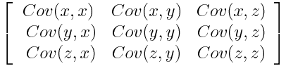
Step 2: Covariance Matrix Computation
The main aim of this step is to understand how the variables of the input data set vary from the mean with respect to each other, that is, to determine if there exists any relationship between them. The covariance matrix is a [n × n] symmetric matrix (where n is the number of dimensions) that has as entries the covariances related to all possible pairs of the initial variables.
What do the covariance matrix entries tell us about the correlations between the variables?
It is actually the sign of the covariance that matters :
if the sign is positive: the two variables increase or decrease together (correlated)
if the sign is negative: One variable increases when the other decreases (Inversely correlated)
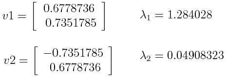
Step 3: Computing the eigenvectors and eigenvalues of the covariance matrix.
Eigenvectors and eigenvalues are the linear algebra concepts, which are required to be computed from the covariance matrix to determine the principal components of the data, which are the "new" variables that are formed from linear combinations or mixtures of the initial variables in our feature set.
Let's assume that the eigenvectors and values of the covariance matrix of our data set are 2-dimensional with two variables (x,y) are as follows:
Step 4: Creation of a feature vector
In this step, we decide if we want to keep all these attributes or discard those of lesser significance (i.e., of low eigenvalues) and, with the help of the remaining ones, form a matrix of vectors that we call Feature vectors.
This will reduce the dimensions of our feature set because if we choose to keep only p eigenvectors (components) out of n, the final data set will have only p dimensions.
Step 5: Recast the data along the axes of the principal component
In this step, we use the feature vector formed using the eigenvectors of the covariance matrix to reorient the data from the original axes to those represented by the principal components (hence the name Principal Components Analysis). To do this, we multiply the transpose of the original data set by the transpose of the feature vector.
Advantages and Disadvantages of Principal Component Analysis
Advantages of PCA
Dimensionality Reduction: PCA transforms a large number of variables into a smaller set of uncorrelated variables called principal components. This reduction simplifies the complexity of the data and facilitates interpretation.
Feature Extraction: It identifies patterns and relationships in data, extracting important features that contribute most to its variance. This helps in focusing on significant components rather than noise.
Multicollinearity Handling: PCA resolves multicollinearity issues by transforming correlated variables into a set of linearly uncorrelated components. This improves the stability and reliability of models.
Improves Model Performance: By reducing noise and focusing on important components, PCA can enhance the performance of machine learning algorithms, especially in cases where the original dataset is high-dimensional.
Data Visualization: PCA allows visual representation of data in reduced dimensions, aiding in exploratory data analysis and understanding the underlying structure of data.
Disadvantages of PCA
Loss of Interpretability: After transformation, the principal components often lose their original meaning in terms of the original variables, making it challenging to interpret the results.
Assumption of Linearity: PCA assumes that the relationships among variables are linear. If the data is non-linear, PCA may not capture the underlying relationships effectively.
Sensitive to Outliers: PCA is sensitive to outliers because it focuses on maximizing variance, which can be disproportionately influenced by extreme values in the data.
Large Computation Costs: Computing PCA requires significant computational resources, especially for large datasets with numerous variables. This can be impractical in some real-time or resource-constrained applications.
Overfitting Risk: In some cases, reducing dimensionality with PCA can lead to overfitting, especially if the number of principal components retained is not chosen carefully relative to the variance explained.
Frequently Asked Questions
When should we use Principal component analysis (PCA)?
When we want to reduce the number of variables, we aren't able to identify the variables which can be removed entirely from consideration.
When we want to ensure your variables are independent of one another
If we're going to make our independent variables less interpretable
What are the limitations of Principal component analysis (PCA)?
Even though principal components are the linear combination of the attributes of the original variables, they are not very easy to interpret.
It's a trade-off between information loss and dimensionality reduction.
What type of data should be used for Principal component analysis (PCA)?
Principal component analysis (PCA) works best on a data set having three or more dimensions. Because, with more dimensions, it becomes increasingly challenging to make interpretations from the resultant cloud of data.
Conclusion
If we have a lot of independent variables to handle, we use Principal component analysis (PCA)to reduce the dimensions of our feature set.
The principal component analysis is a technique, which combines our input variables through their linear combinations and mixtures, and then we can drop the "least significant" variables while still retaining the most valuable attributes of all of the variables.


 8+ registered

