ResNet Architecture

Why is ResNet used?

To get better accuracy from a deep learning model, we use more and more layers. By adding more layers, we can learn more about the complex features of the input. This works for fewer layers, but as we keep on increasing the number of layers, we are faced with problems such as vanishing gradient or exploding gradient. Vanishing gradient is caused when the gradient becomes close to zero. If the gradient becomes too large, it is known as exploding gradient. This decreases the accuracy of the model. 

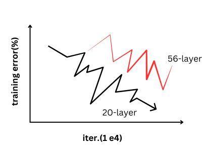
While training the deep learning model, the gradient is backpropagated to the previous layers. As we increase the number of layers, the gradient becomes very small due to repeated multiplication, and its performance is decreased.

We can see above, The 56 layered model is giving higher error than the 20 layered model both in training and in test data. It is not due to overfitting because the training error is also high. This problem was mitigated by the arrival of ResNet. 

Residual blocks: The building blocks of ResNet

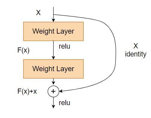
Residual blocks are the building blocks of ResNet. Let us look at these residual blocks.

We can understand the structure of the residual blocks from the above image. As we can see, there is a direct connection between some layers, which skips the in-between layers. This is called skip connection and is the core of residual blocks. Due to these skip connections, the output is changed.

Without these skip connections, the input (X) is passed through all the layers in between and is multiplied by the corresponding weights of the layer and then added by a bias term. Then it goes through an activation function to give us the final outcome.

The authors of the original paper state this as “Formally, denoting the desired underlying mapping as H(x), we let the stacked nonlinear layers fit another mapping of F(x) := H(x)−x. The original mapping is recast into F(x)+x.”^[1] 

Sometimes the dimensions of the input differ from that of the output. To overcome this, we can:

1. We can use padding in the skip connections to increase their dimensions 
2. We can add 1X1 convolutional layers to the input. This method is called the projection method.

 

Any layer that decreases the performance of the model is skipped due to regularization.

ResNet Architecture

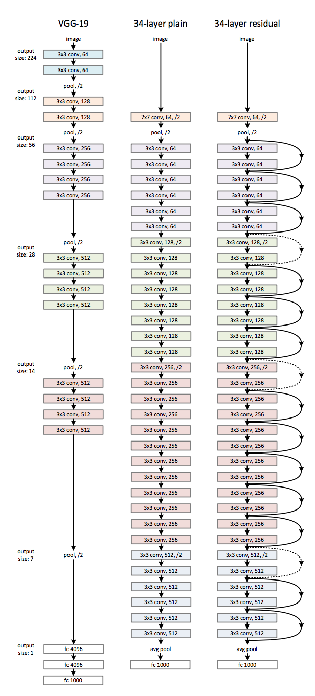
ResNet takes a 34 layered plain architecture and then adds then skips the connections in between the layers. The plain architecture is inspired by VGG-19. Below is a visual representation of ResNet.

Variations of ResNet

After the huge success of ResNet, it was researched thoroughly, and some new variants of ResNet were created. Let us look at some of these variants of ResNet.

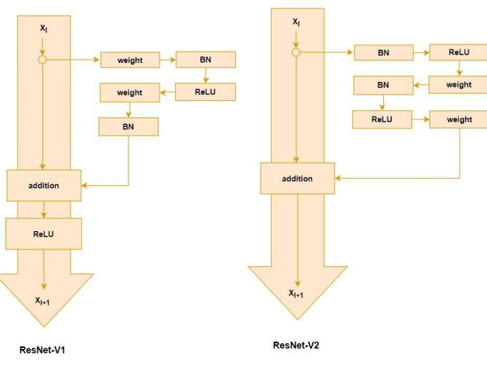
There are mainly two versions of ResNet, ResNet version 1 ( ResNet-V1) and ResNet version 2 (ResNet-V2).

ResNet-V1 adds a second non-linearity after the addition of F(X) and X. ResNet-V2, on the other hand, removed this non-linearity.

ResNet-V1 performs convolution after the batch normalization and ReLU activation. ResNet-V2 uses Batch Normalization and ReLU activation to the input before its multiplication with the weight(W) matrix.

Difference between ResNet-V1 and ResNet-V2

The main difference between ResNet-V2 and ResNet-V1 is that ResNet-V2 uses batch normalization before each weight layer.

ResNET -V1	ResNET -V2
y= xl + F( xl , {Wi}) xl+1=H(x) = ReLU(y)	y = h(xl) + F(xl, {Wi}) xl+1=H(x) = f(y)
y= Additional Output xl+1 = Input to Next Block	y= Additional Output h(xl) = Generalized form of input              For Resnet V1, h(xl) = xl f = Function applied to ‘y’      For Resnet V1, f = ReLU        For Resnet V2, f is an identity mapping.

We have ResNet architectures that use different layers for the same concept. We have ResNet-50, ResNet-101, ResNet-110, ResNet-152, ResNet-164, ResNet-1202, etc. The two digits followed by ResNet give us the number of layers used. For example, ResNet-50 means ResNet architecture with 50 layers.

There are also some interpretations of ResNet that use the ‘skip layer’ concept. For example, DenseNet, and Deep Network with Stochastic Depth.

Implementing ResNet using Keras

Keras provides support for the following versions of ResNet:

1. ResNet50
2. ResNet50V2
3. ResNet101
4. ResNet101V2
5. ResNet152
6. ResNet152V2

Let us implement ResNet50 by using Keras:

Importing the library:

from keras.applications.resnet50 import ResNet50

 

We will download a base model that has ResNet50 architecture with pre-trained weights

base_model = ResNet50(include_top=False, weights='imagenet')

 

Adding a fully connected layer having 2048 neurons with ReLU activation

x = Dense(2048, activation='relu')(x)

 

Adding a fully connected layer that will classify the input. The number of neurons depends on the number of classifications that we want to have. For example, if we want to classify our input to give the probability of it being either a car or a truck. The layer will be:

predict = Dense(2, activation='softmax')(x)

 

The final model that we want to train:

model = Model(inputs=base_model.input, outputs=predict)

 

The training data and the test data will be provided by us. We will have to provide the path to the training and the test set, set the target size, and the batch size. An example of how we can prepare our training dataset for training:

training_set = train_datagen.flow_from_directory('training_set',
                                                target_size = (224, 224),
                                                batch_size = 48,
                                                class_mode = 'categorical')

 

Training the model for 50 epochs:

model.fit_generator(training_set,
                        steps_per_epoch = 9000,
                        epochs = 50,
                        validation_data = test_set,
                        validation_steps = 3000)

 

We can save the weights in the current directory by using:

model.save_weights("resnet50_weights.h5")

 

To get the predictions:

test_image = “..location-of-the-image/image.jpg”
result = classifier.predict(test_image)

 

                       Test image

                        Prediction

What is the difference between ResNet and ResNet50?

Aspect	ResNet	ResNet50
Architecture	Basic Residual Network architecture	Residual Network with 50 layers
Depth	Typically has fewer layers (e.g., 18)	Specifically designed with 50 layers
Parameters	Fewer parameters	More parameters for deeper networks
Performance	Suitable for simpler tasks	Suitable for complex tasks
Computational	Requires less computational resources	Requires more computational resources
Usage	Used in less complex applications	Commonly used in deep learning tasks

Frequently Asked Questions

How is padding applied to the skip layer?

The skip connection is padded with zeroes to increase its dimensions.

What are the practical benefits of ResNet?

We can load a pre-trained version of the network trained on over a million images and can easily use it to classify our images on over 1000 categories.

Is ResNet a CNN or RNN?

ResNet is a CNN.

Conclusion

This article was an exhaustive look at ResNet. We talked about the fantastic results shown by ResNet. We also talked about why it is needed and its benefits. After that, we dived deeper into ResNet and looked into the concept behind it and its different variants. Finally, we understood how it could be implemented in our code using Keras. You can read the original paper on ResNet here.

Refer to our Guided Path on Coding Ninjas Studio to upskill yourself in Data Structures and Algorithms, Competitive Programming, JavaScript, System Design, Machine learning, and many more! If you want to test your competency in coding, you may check out the mock test series and participate in the contests hosted on Coding Ninjas Studio! But if you have just started your learning process and are looking for questions asked by tech giants like Amazon, Microsoft, Uber, etc. You must look at the problems, interview experiences, and interview bundle for placement preparations.

Nevertheless, you may consider our paid courses to give your career an edge over others!

Do upvote our blogs if you find them helpful and engaging!