Do you think IIT Guwahati certified course can help you in your career?
Introduction
Computers must understand pictures and find common patterns, so we must revise some methods. These methods need to include essential information that makes sense of the images. To solve this, we create deep networks with many layers, which can identify simple and complex features in pictures. This way, the whole system can learn better. However, deep networks encounter the "vanishing gradients" problem, where early layers become too small to make a difference. ResNet, a new network type, was introduced to solve this problem.
In this article, we will discuss ResNet in PyTorch. We will also explore its architecture and comparison with other CNN architectures.
PyTorch
PyTorch is a tool that supports developers in working with deep learning models. It includes numerous helpful features for creating and training neural networks. One wonderful thing about it is its dynamic computational graph, which makes fixing errors and flexibly developing models effortless. Developers like PyTorch more than TensorFlow because it operates on simple and familiar Python commands. Also, many people support and enhance PyTorch, so it's widely used in the AI and machine learning community.
ResNets
ResNet, which stands for "Residual Network," is a deep neural network that significantly changed how computers recognize images. The wonderful thing about ResNet is that it utilizes "residual blocks" to understand the difference between what goes in and what emerges from each layer. It makes it easier to train deep networks, making them more accurate in understanding images. Because of ResNet, we can now create better computer programs for tasks like recognizing objects in pictures, finding things in photos, splitting snaps into different parts, and even generating new images. It has become one of the famous and successful deep learning models.
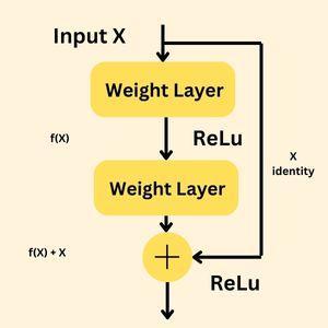
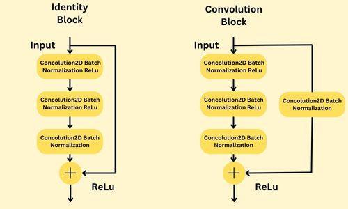
Residual Block
In ResNet, a "residual block" serves as a building block for the whole network. It includes multiple layers stacked together. Here's the exciting part: we add the output of one layer to another layer deeper inside the block. Then, they use a particular function to combine the results. This direct connection between layers is called a "shortcut" or "skip connection." These shortcuts enable the network to learn better and make it possible to train intense networks effectively. It's like solving a tricky problem called the "vanishing gradient." Because of these shortcuts, ResNet is excellent at identifying images and works well in computer tasks like object recognition.
Implementation of ResNet
Let's take a step-by-step example to understand the working of ResNet better.
Importing the Libraries
In the first step, we will import all the required libraries such as Numpy for numerical computations, Torch for deep learning framework in the PyTorch, 'torch.nn' module that has tools for constructing a neural network, transform for image transformation to perform computer vision and SubsetRandomSampler to select random sample data from a provided dataset.
Python
Python
import numpy as np
import torch
import torch.nn as nn
from torchvision import datasets
from torchvision import transforms
from torch.utils.data.sampler import SubsetRandomSampler

# Device configuration
device = torch.device('cuda' if torch.cuda.is_available() else 'cpu')
You can also try this code with Online Python Compiler
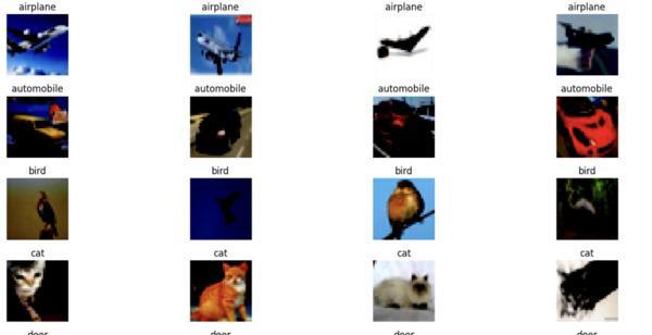
In the second step, we must load our dataset into the system. To load our dataset, we use a library called torchvision. It allows us to effortlessly access numerous computer vision datasets and preprocess them for modeling. We define a function called "data_loader" to return the training or test data based on the input.
Python
Python
def data_loader(data_dir,
batch_size,
random_seed=42,
valid_size=0.1,
shuffle=True,
test=False):
# Normalize the dataset with mean and standard deviation
normalize = transforms.Normalize(
mean=[0.4914, 0.4822, 0.4465],
std=[0.2023, 0.1994, 0.2010],
)
# Define transforms
transform = transforms.Compose([
transforms.Resize((224,224)),
transforms.ToTensor(),
normalize,
])
if test:
# Load the test dataset
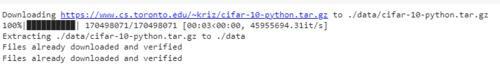
dataset = datasets.CIFAR10(
root=data_dir, train=False,
download=True, transform=transform,
)
# Create a data loader for the test dataset
data_loader = torch.utils.data.DataLoader(
dataset, batch_size=batch_size, shuffle=shuffle
)
return data_loader
# load the training and validation datasets
train_dataset = datasets.CIFAR10(
root=data_dir, train=True,
download=True, transform=transform,
)
valid_dataset = datasets.CIFAR10(
root=data_dir, train=True,
download=True, transform=transform,
)
num_train = len(train_dataset)
indices = list(range(num_train))
split = int(np.floor(valid_size * num_train))
if shuffle:
np.random.seed(42)
np.random.shuffle(indices)
# Split the training dataset
train_idx, valid_idx = indices[split:], indices[:split]
train_sampler = SubsetRandomSampler(train_idx)
valid_sampler = SubsetRandomSampler(valid_idx)
train_loader = torch.utils.data.DataLoader(
train_dataset, batch_size=batch_size, sampler=train_sampler)
valid_loader = torch.utils.data.DataLoader(
valid_dataset, batch_size=batch_size, sampler=valid_sampler)
return (train_loader, valid_loader)
# CIFAR10 dataset
train_loader, valid_loader = data_loader(data_dir='./data',
batch_size=64)
test_loader = data_loader(data_dir='./data',
batch_size=64,
test=True)
You can also try this code with Online Python Compiler
Then we normalized the dataset by calculating each color channel's mean and standard deviation. Data loaders are helpful because they allow us to examine and pass the data in small batches. It is useful when dealing with large datasets with millions of pictures.
Build Residual Block
To begin constructing the network, we build a ResidualBlock that we can reuse throughout the entire network. This block includes a special "skip connection" , an optional parameter. The skip connection allows the input "x" to join the block output directly. This ResidualBlock will create our network more efficiently and uncomplicated to train by allowing residual learning.
Python
Python
class CodingNinjasResidualBlock(nn.Module):

    # Set parameters and attributes
    def __init__(self, cn_in_channels, cn_out_channels, cn_stride=1, cn_downsample=None):
        super(CodingNinjasResidualBlock, self).__init__()

        # First convolutional layer
        self.cn_conv1 = nn.Sequential(
            nn.Conv2d(cn_in_channels, cn_out_channels, kernel_size=3, stride=cn_stride, padding=1),
            nn.BatchNorm2d(cn_out_channels),
            nn.ReLU()
        )

        # Second convolutional layer
        self.cn_conv2 = nn.Sequential(
            nn.Conv2d(cn_out_channels, cn_out_channels, kernel_size=3, stride=1, padding=1),
            nn.BatchNorm2d(cn_out_channels)
        )
        self.cn_downsample = cn_downsample
        self.cn_relu = nn.ReLU()
        self.cn_out_channels = cn_out_channels

    def forward(self, x):
        residual = x
        out = self.cn_conv1(x)
        out = self.cn_conv2(out)
        if self.cn_downsample:
            residual = self.cn_downsample(x)
        out += residual
        out = self.cn_relu(out)
        return out
You can also try this code with Online Python Compiler
Now that we keep our ResidualBlock ready, we can build our ResNet, a robust deep-learning architecture for image classification. To construct each block, we operate a helper function called _make_layer. This operation adds the layers individually, including the ResidualBlock, as needed.
After finishing the blocks, we add an average pooling layer to lower the spatial dimensions further. Ultimately, we encompass the final linear layer that produces the outcome for each category in our image classification task.
Python
Python
class CodingNinjasResNet(nn.Module):
    # Set the parameters and attributes
    def __init__(self, cn_block, cn_layers, cn_num_classes=10):
        super(CodingNinjasResNet, self).__init__()
        self.cn_inplanes = 64
        self.cn_conv1 = nn.Sequential(
            nn.Conv2d(3, 64, kernel_size=7, stride=2, padding=3),
            nn.BatchNorm2d(64),
            nn.ReLU()
        )
        self.cn_maxpool = nn.MaxPool2d(kernel_size=3, stride=2, padding=1)
        self.cn_layer0 = self._make_layer(cn_block, 64, cn_layers[0], stride=1)
        self.cn_layer1 = self._make_layer(cn_block, 128, cn_layers[1], stride=2)
        self.cn_layer2 = self._make_layer(cn_block, 256, cn_layers[2], stride=2)
        self.cn_layer3 = self._make_layer(cn_block, 512, cn_layers[3], stride=2)
        self.cn_avgpool = nn.AvgPool2d(7, stride=1)
        self.cn_fc = nn.Linear(512, cn_num_classes)
    # Acts like a helper function to create a sequence of residual blocks in a layer
    def _make_layer(self, cn_block, cn_planes, cn_blocks, stride=1):
        cn_downsample = None
        if stride != 1 or self.cn_inplanes != cn_planes:
            cn_downsample = nn.Sequential(
                nn.Conv2d(self.cn_inplanes, cn_planes, kernel_size=1, stride=stride),
                nn.BatchNorm2d(cn_planes),
            )
        layers = []
        layers.append(cn_block(self.cn_inplanes, cn_planes, stride, cn_downsample))
        self.cn_inplanes = cn_planes
        for i in range(1, cn_blocks):
            layers.append(cn_block(self.cn_inplanes, cn_planes))
        return nn.Sequential(*layers)
    def forward(self, x):
        x = self.cn_conv1(x)
        x = self.cn_maxpool(x)
        x = self.cn_layer0(x)
        x = self.cn_layer1(x)
        x = self.cn_layer2(x)
        x = self.cn_layer3(x)
        x = self.cn_avgpool(x)
        x = x.view(x.size(0), -1)
        x = self.cn_fc(x)
        return x

# Example usage:
# Instantiate the CodingNinjasResNet
cn_resnet = CodingNinjasResNet(CodingNinjasResidualBlock, [2, 2, 2, 2], cn_num_classes=10)

# Generate a random input tensor (batch_size=1, 3 channels, 224x224 image)
input_tensor = torch.randn(1, 3, 224, 224)

# Pass the input tensor through the model
output = cn_resnet(input_tensor)

# Print the output shape
print("Output shape:", output.shape)
You can also try this code with Online Python Compiler
You set the parameter according to your need. We must experiment with different hyperparameter values for our model to discover the most suitable setting. The hyperparameters specify the number of epochs, batch size, learning rate, loss function, and optimizer.
Python
Python
cn_num_classes = 10
cn_num_epochs = 20
cn_batch_size = 16
cn_learning_rate = 0.01
cn_model = CodingNinjasResNet(CodingNinjasResidualBlock, [3, 4, 6, 3]).to(device)

# Loss and optimizer
cn_criterion = nn.CrossEntropyLoss()
cn_optimizer = torch.optim.SGD(cn_model.parameters(), lr=cn_learning_rate, weight_decay=0.001, momentum=0.9)

# Train the model
cn_total_step = len(cn_train_loader)
You can also try this code with Online Python Compiler
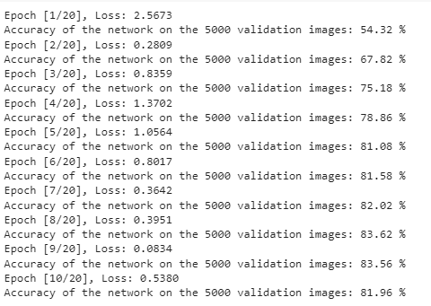
In the training method of our model in PyTorch, we load pictures in batches using the train_loader. The model forecasts labels for these images, and we estimate the loss between the predictions and the actual labels using the loss function. After each training epoch, we estimate the model on the validation set and turn off gradient measures to speed up the evaluation process. Following these steps, we iteratively train the model to better execute our image classification task.
Python
Python
import gc

cn_total_step = len(cn_train_loader)

for cn_epoch in range(cn_num_epochs):
    for cn_i, (cn_images, cn_labels) in enumerate(cn_train_loader):
        cn_images = cn_images.to(device)
        cn_labels = cn_labels.to(device)

        # Forward passing
        cn_outputs = cn_model(cn_images)
        cn_loss = cn_criterion(cn_outputs, cn_labels)


        # Backward passing and optimization
        cn_optimizer.zero_grad()
        cn_loss.backward()
        cn_optimizer.step()
        del cn_images, cn_labels, cn_outputs
        torch.cuda.empty_cache()
        gc.collect()

    print('Epoch [{}/{}], Loss: {:.4f}'
          .format(cn_epoch + 1, cn_num_epochs, cn_loss.item()))


     with torch.no_grad():
        cn_correct = 0
        cn_total = 0
        for cn_images, cn_labels in valid_loader:
            cn_images = cn_images.to(device)
            cn_labels = cn_labels.to(device)
            cn_outputs = cn_model(cn_images)
            _, cn_predicted = torch.max(cn_outputs.data, 1)
            cn_total += cn_labels.size(0)
            cn_correct += (cn_predicted == cn_labels).sum().item()
            del cn_images, cn_labels, cn_outputs


print('Accuracy of the network on the {} validation images: {} %'.format(5000, 100 * cn_correct / cn_total))
You can also try this code with Online Python Compiler
Below is a comparison of ResNet with other CNN architectures.
Architecture
Year
Features
Use cases
LeNet
1998
LeNet was the first application of CNN.
It uses a sigmoid or tanh activation function.
It is mostly used in handwritten digit recognition.
AlexNet
2012
AlexNet was the first that used ReLu activation.
It used GPU to train its model.
It is mainly used in image recognition.
VGGNet
2014
VGGNet is a deep network with small convolutional filters.
It has many configurations, such as VGG16 or VGG19.
It is used in image recognition.
ResNet
2015
ResNet uses Residual connections to tackle vanishing gradients.
It introduces "skip connections" or "shortcuts."
It has many configurations like ResNet-50, ResNet-101 or ResNet-152.
It is mostly used in large-scale image recognition.
GoogleLeNet
2014
GoogleLeNet uses inception modules for multi-scale features.
It has many versions like Inception v1, v2 or v3.
It is primarily used in image classification and object recognition.
Frequently Asked Questions
What in PyTorch is ResNet?
ResNet is a deep neural network architecture in PyTorch created to overcome the vanishing gradient problem by using skip connections or residual blocks.
Using skip connections, how does ResNet work?
ResNet uses skip connections to directly propagate the input across multiple layers during training, facilitating the gradient flow.
What are residual blocks in ResNet?
The essential building components of ResNet are residual blocks. Each block has a shortcut link combining the original input with a group of convolutional layers.
What issue is resolved by ResNet architecture?
ResNet addresses the degradation issue by enabling very deep networks (with more than 100 layers) to train without worrying about disappearing gradients.
How is the architecture of ResNet categorized?
The ResNet architectures group their many layers, such as ResNet-18, ResNet-34, ResNet-50, etc. The number reflects the total number of layers, which includes convolutional and fully connected layers.
Conclusion
In this article, we learned about ResNet in PyTorch. We also realized some unique features of PyTorch that attract developers to operate it. We even examine the term residual block and why it is crucial. To understand better about ResNet, we implemented the ResNet on a sample dataset and discovered its accuracy. We also compared ResNet and other architectures like VGGNet or AlexNet to understand what makes ResNet so special.
Do check out the link to learn more about such topic
You can find more informative articles or blogs on our platform. You can also practice more coding problems and prepare for interview questions from well-known companies on your platform, Coding Ninjas Studio.


 9+ registered

