RMSProp
RMSProp stands for Root Mean Square Propagation. RMSprop is an optimization technique that we use in training neural networks. RMSProp was first proposed by the father of back-propagation, Geoffrey Hinton.
The gradients of complex functions like neural networks tend to explode or vanish as the data propagates through the function (known as vanishing gradients problem or exploding gradient descent). RMSProp was developed as a stochastic technique for mini-batch learning.
RMSprop deals with the above issue by using a moving average of squared gradients to normalize the gradient. This normalization balances the step size (momentum), decreasing the step for large gradients to avoid exploding and increasing the step for small gradients to avoid vanishing.
In simple terms, RMSprop uses an adaptive learning rate instead of treating the learning rate as a hyperparameter. This means that the learning rate varies over time. RMSprop uses the same concept of the exponentially weighted average of gradient as gradient descent with momentum, but the difference is parameter update.
Parameters Updation
The recursive formula of EWA is given by:
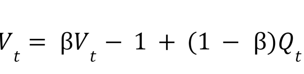
Where,
Vt: Moving average value at t.
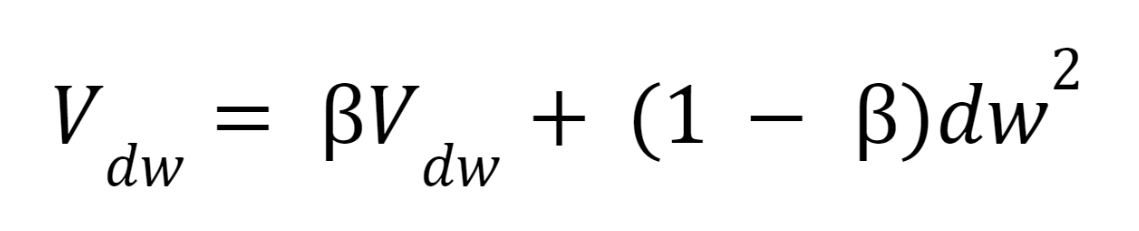
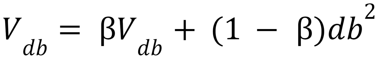
In RMSProp, we find the EWA of gradients and update our parameters using those EWAs. On each iteration t, we calculate dw and db on the current minibatch. Then we calculate vdw and vdb using the following formulae:
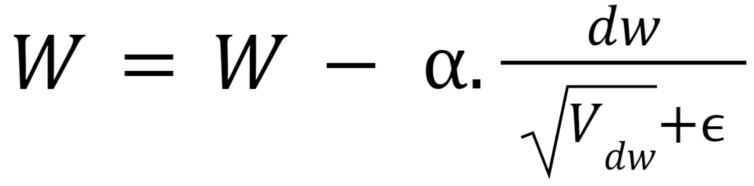
We will update our parameters after calculating the exponentially weighted averages.
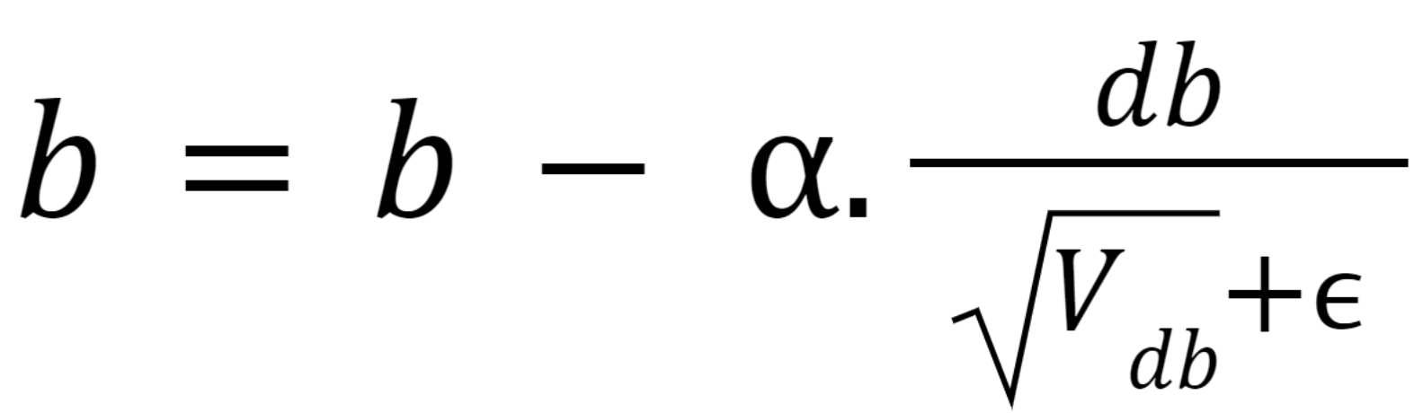
W = W - learning rate * dW
b = b - learning rate * db.
Putting the value of db and dw in respective equations, we get:
We try to diminish the vertical movement using the average because they sum up to 0(approximately) while averaging.
Ideal Values of Alpha and Beta
The suggested value of β is 0.9, which is observed experimentally. If we keep β lesser than 0.9, then the fluctuation in the value of vdw and vdb will be very high. On the other hand, keeping the value of β higher than 0.9 will not give a proper value for average.
The suggested value of alpha is 0.001. Keeping alpha less than 0.001 will make the learning slower, whereas keeping it more than 0.001 will generate the chance of overshooting the minima.
Working Of RMSProp
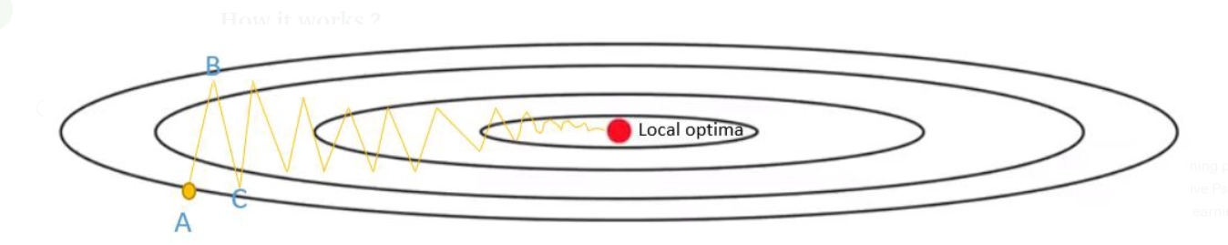
We start gradient descent from point A. After one iteration of gradient descent, we may end up at point B. Then another gradient descent step may end up at point C. After some iteration, we step towards the local optima with oscillations up and down. Using a higher learning rate would make the vertical oscillation frequency more significant, slowing our gradient descent. Thus, using a higher learning rate is prevented.
The bias plays a role in determining the vertical oscillations, whereas the weight defines the movement in the horizontal direction. If we slow down the updatation process for bias, then the vertical oscillations can be dampened, and if we update ‘weights’ with higher values, we can still move quickly towards the local optima.
We require to slow down the learning in the vertical direction and boost up or at least not slow down the learning in the horizontal direction. i.e., in the horizontal direction, we want to move fast, and in the vertical direction, we want to slow down or damp out the oscillation.
The derivative db is much larger in the vertical direction than dw in the horizontal direction. So because of this Vdw will be small, and Vdb will be larger, and hence the updates will be slowed down in vertical directions.
Talking about the net effect of RMSProp, the vertical direction movement is reduced because reaching the minimum point is quick and learning of the parameters isis much faster than the earlier cases.
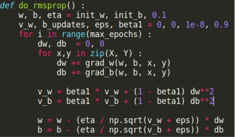
Implementation
Img_src
Frequently Asked Questions
-
Is RMSProp stochastic gradient descent?
RMSProp lies in the adaptive learning rate methods region, growing in popularity in recent years. It is the extension of the Stochastic Gradient Descent (SGD) algorithm, momentum method, and the foundation of the Adam algorithm.
-
Is Adam better than RMSProp?
Currently, Adam is a little bit better than RMSProp. However, we can also try using SGD with Nesterov Momentum as an alternative.
-
What is the reason for using an RMSProp optimizer?
The RMSprop optimizer minimizes the oscillations in the vertical direction. So, we can increase our learning rate, and our algorithm could take larger steps in the horizontal direction converging faster.
-
Who invented RMSprop?
RMSprop— is an unpublished optimization algorithm designed for neural networks, first proposed by Geoff Hinton.
-
What is the difference between RMSprop and Adam?
While momentum accelerates our search in direction of minima, RMSProp impedes our search in direction of oscillations. Adam combines the heuristics of both Momentum and RMSProp.
Key Takeaways
Let us brief the article.
Firstly we saw the reason behind using RMSProp, the need for RMSProp, and have a detailed study about RMSProp. We saw how the parameters get updated and the working behind of RMSPRop. Lastly, we saw the ideal alpha and beta values and ended the article with python implementation.
RMSprop is a good, fast, and very popular optimizer. It learns properly and tunes the internal parameters to minimize the Cost function. Root Mean Square Propagation(RMSProp) is one of the most popular optimization algorithms we use in deep learning. Adam only surpasses its popularity. So, RMSProp is an excellent alternative to Gradient Descent.
I hope you all like this article.
Happy Learning Ninjas!


 9+ registered

