Round Robin Scheduling

Introduction 

One fine day you are chatting with your friends while working on the same device. Now you wanted to listen to some soothing music, you opened Youtube and started listening to music. So, you are performing three activities on a single device. Cool, but have you ever wondered how things are going on the backend?

How is your system managing to multitask? 

Well, that’s worth thinking about the scheduling process going on in the backend. To simply explain, every activity is considered the Process. And to execute each process efficiently, the CPU utilizes some scheduling algorithms, one of which is the Robin Round algorithm. 

Before we get further into the algorithm, let's look back at where it came from. Round Robin is the most basic and oldest scheduling algorithm. The algorithm's name is derived from the round-robin principle, which states that each individual receives an equal amount of something in turn. 

Recommended Topic, FCFS Scheduling Algorithm, Multiprogramming vs Multitasking

What is Round-Robin(RR) Scheduling?

The Round Robin (RR) scheduling algorithm is primarily intended for use in time-sharing systems. This approach is similar to FCFS scheduling; however, Round Robin(RR) scheduling incorporates preemption, allowing the system to switch between processes. Preemption enables the process to be forcefully taken out of the CPU. 

How exactly does it work? 

• A fixed time slice is associated with each request, known as the Time Quantum. 
• The job scheduler saves the progress of the job that is being executed currently and moves to the next job present in the queue when a particular process is executed for a given time quantum. 
• No process will hold the CPU for a long time, making RR scheduling efficient. Yet again, it depends on the chosen time for the quantum. We’ll see how fluctuation in the time quantum leads to more/less context switching later in this article itself. 

Important terms to understand Round Robin Scheduling 

1. Burst Time

Every process in a computer system necessitates time for its execution.  This time includes both CPU and I/O time. The CPU time is the time it takes the CPU to perform the process. The I/O time, on the other hand, is the time it takes the process to do an I/O activity. We generally disregard I/O time and solely evaluate CPU time for a process. As a result, burst time is the entire time required by the process to execute on the CPU.

2. Arrival Time 

As the name implies, Arrival time is when a process enters the ready state and is ready to be executed.

3. Exit Time/Completion Time

The time when a process completes its execution and exits the system is called exit time.

4. Turn Around Time 

The total time spent by the process from coming in the ready state for the first time to its completion is referred to as Turnaround Time. 

This mostly represents the time difference between completion and arrival. The formula for calculating is as follows: 

Turnaround Time = Completion Time - Arrival Time

5. Waiting Time 

The cumulative time spent by the process in the ready state waiting for the CPU is referred to as waiting time. 

It represents the time difference between the turnaround and the burst time. 

Waiting Time = Turn Around Time – Burst Time

Example of Round-Robin Scheduling

Let us now take an example to understand how exactly the Round Robin Scheduling algorithm works: 

Time Quantum: 2 ms. 

In the above example, we’ve given the arrival time and the burst time. Since we are focusing on the RR scheduling, the execution is as follows: 

To perform the scheduling, we require a Queue and a Gannt chart. 

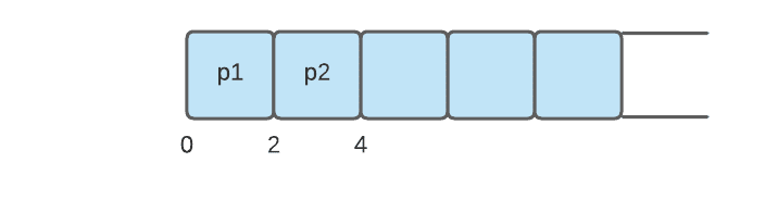
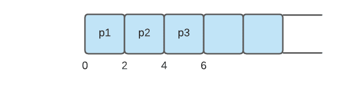
Step 1: The execution begins with process P1, with a burst time of 3. Here every process executes for 2 miliseconds. The Gannt chart and the Queue will look like this: 

Queue: 

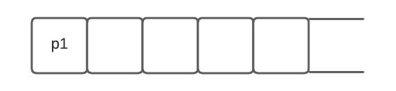
Gantt chart: 

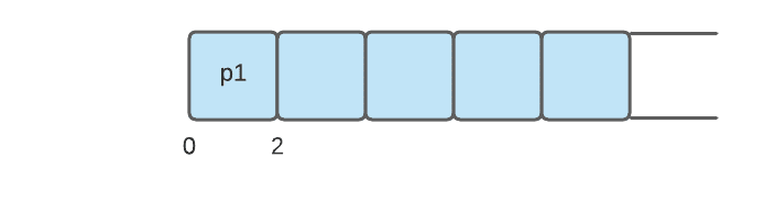
As we can see, P1 is still left with 1ms. We can say that its execution is not yet completed. 

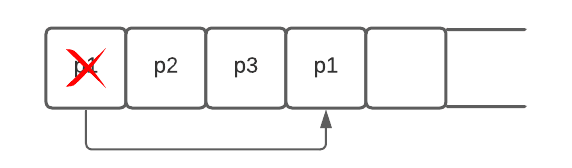
At the time of 2 sec, another process must have arrived. From the above table, P2(AT = 1) and P3(AT = 2) will be in the queue as shown below:

P1 is not yet completed since it has exceeded the time slice; it will be moved at the end of the queue, and the other processes will be executed. 

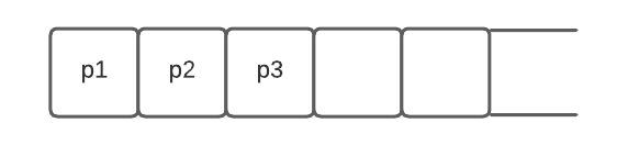
Step 2: The next step is to execute the following processes. The process P2, burst time 4, will be executed next. 

Gantt Chart: 

Other processes would have arrived; in our case, it will be the process P4(AT= 3). Hence the queue will look like this: 

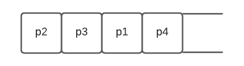
Since the process, P2 has 2 ms left, and it is not yet completed will be moved at the end of the queue. 

Step 3: The process P3 will be executed next with the burst time = 2. The Gannt chart will look like this:

Gantt chart: 

Since it is completed with the execution due to its having the same burst time as the time quantum, it will be discarded from the queue. 

Step 4: The following process that is P1, will be executed now, which has 1ms burst time left. Here, the time quantum is greater than the burst time. In such cases, minimum time will be considered. 

Gantt chart: 

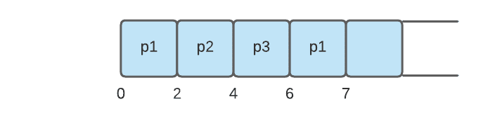
Simultaneously it will be discarded from the queue. 

Step 5: The following process in the queue is P4 which has the burst time = 1. Likewise, in the above case, the minimum time will be considered. 

Gantt Chart: 

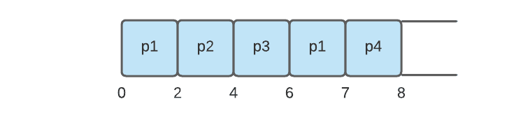
The process P4 now will be discarded from the queue. 

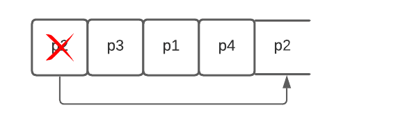
Step 6: The process P2 will be executed next, with the burst time left = 2ms. 

Gantt chart: 

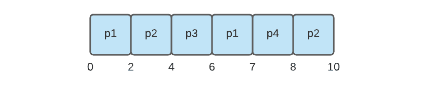
The queue will be empty now. 

Now we need to find several terms: 

1. Completion time: Completion time will be calculated from the Gantt chart: 

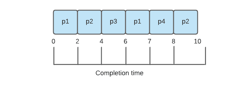
The scanning goes from right to left. 

For P1: 7 

For P2: 10

For P3: 6

For P4: 8 

2. Turn Around Time: Completion Time - Arrival Time 

For P1: 7- 0 = 7

For P2: 10 - 1 = 9

For P3: 6 - 2 = 4

For P4: 8 - 3 = 5 

3. Waiting Time: Turn Around Time - Burst Time 

For P1: 7 - 3 = 4

For P2: 9 - 4 = 5

For P3: 4 - 2 = 2

For P4: 5 -  1 = 4

Flowchart

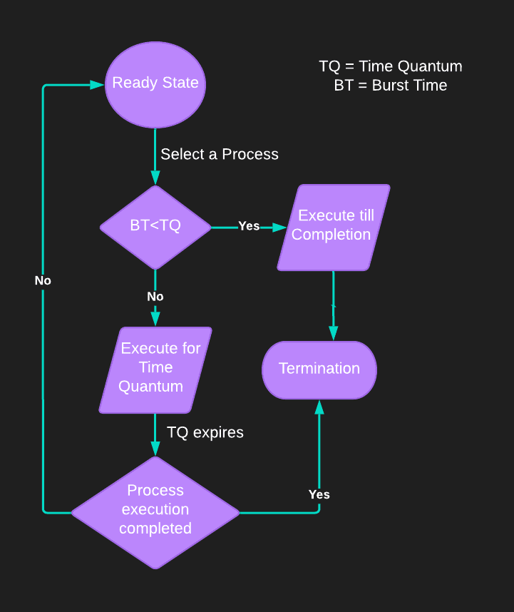
Try out Round Robin Scheduling implementation on your own

Advantages of Round Robin Scheduling 

• Since the CPU serves each process for a fixed time quantum, all processes are assigned the same priority.
• As each round-robin cycle gives each process a predetermined time to run, starvation does not arise. No procedure is overlooked.

Disadvantages of Round Robin Scheduling 

• The choice of the length of the time quantum has a considerable impact on the throughput in RR. If the time quantum is longer than required, it behaves similarly to FCFS.
• If the time quantum is less than required, the number of times the CPU switches from one process to another rises. As a result, CPU efficiency suffers.

Must Read Evolution of Operating System, Open Source Operating System.