Sigmoid Neuron

Data and Task

We can use the sigmoid neuron for both binary classification and regression. The inputs of the sigmoid neuron can be real numbers, unlike the boolean inputs in Multi-layer Perceptron Neuron, and the output will also be an actual number ranging between 0–1. In the sigmoid neuron, we try to regress the relationship between X and Y in terms of probability. Even though we know that the output is between 0–1, we can still use the sigmoid function for binary classification tasks by taking some threshold values.

 

Model

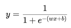
The sigmoid function gives us an "S-shaped function," much smoother concerning 0/1 perceptron. Given X(high dimensional real value input) and Y(real value output between 0-1), the approximate relationship between the two is given by the Sigmoid function.

 

In the case of one-dimensional input X,

 

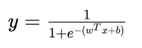
In the case of multi-dimensional input X,

 

Loss Function

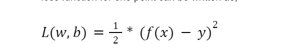
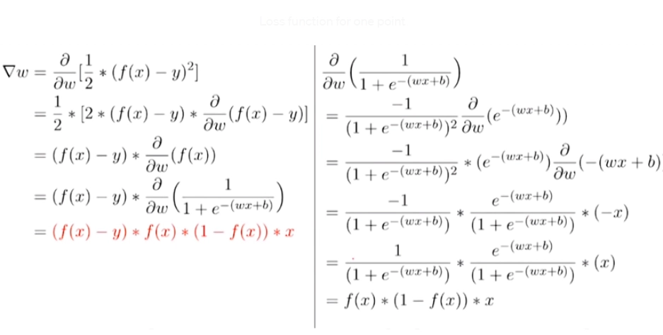
We will use the well-known loss function technique, i.e., the squared error loss function. It is the sum of the square difference between the actual and predicted output.

 

We can use another technique to measure loss function, i.e., Cross-entropy loss function.

 

Learning Algorithm(Gradient Descent)

Under this tag, we will study how an algorithm learns the parameters w and b of the sigmoid neuron model by using a gradient descent model. The main objective of this learning algorithm is to determine the best optimal values of w and b such that the predicted output is as close to the actual output, i.e., minimize the loss function.

 

The learning algorithm looks like this:

Learning Algorithm

 

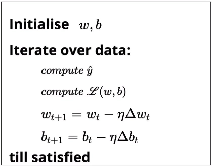
Initially, we randomly chose the value of w and b. We then iterate over the training data inputs. We calculate the predicted outcome using the sigmoid function for each observation, then compute the loss using the loss function(squared-error loss). Based on the loss value, we update the value of the weights and bias, such that the loss due to these new parameters is less than the previous one.

We will keep on repeating the above process until we reach the following three conditions:

• The loss of the model becomes zero.
• We have already performed enough iterations based on the computational capacity.
• The overall loss of the model becomes negligible or closer to zero.

 

If any of the three conditions are met, we stop the process.

 

We saw how the weights are getting updated based on the loss value. This section will know why this specific update rule would reduce the model's loss. To understand why the update work rule works, we need to understand its math.

Maths Behind Learning Algorithm

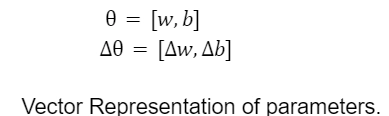
We can represent the two parameters in the sigmoid function in a vector theta. 

 

 

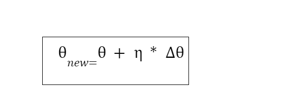
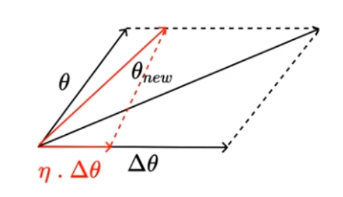
So the geometric representation of theta and new theta. As both are vectors, they should follow the parallelogram vectors law, so the resulting new theta is diagonal of the parallelogram. From the geometrical representation, it is clear that there is a large change between the value of theta and new theta, so to take small conservative steps, we multiply the delta theta with a constant known as the learning rate. So the new theta will have value:

 

 

Geometrical Representation

 

Now the question arises how to decide the value of delta theta? Well, we have to find such value of the new theta such that the loss due to the new theta is less than that of the old theta. The answer to this question is given from the Taylor series.

 

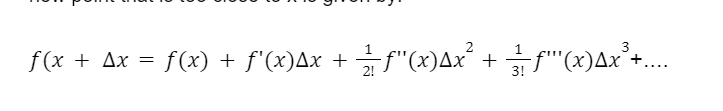
Taylor Series

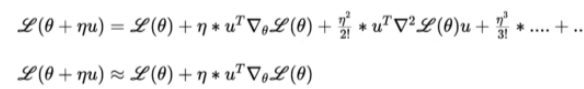
Taylor series states that if we know the values of a function f at x, then the value at a new point that is too close to x is given by:

 

We will now reduce the Taylor series in terms of sigmoid neuron parameters and loss function. For simplicity,  let’s assume delta theta=u, then the equation reduces to,

 

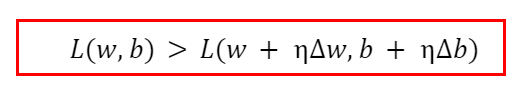
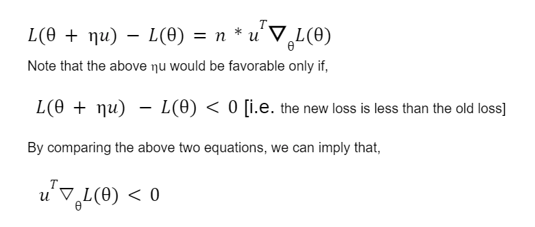
We have to find the optimal value of the change vector uT such that the value after L(theta) turns out to be negative. If the value is negative, we can say that the loss at the new theta is less than the loss at the old theta.

 

For simplicity, let us approximate the above equation as the learning rate  is minimal. Any positive value raised to the learning rate will be too negligible to consider reducing the above Taylor series to the second equation in the above image.

 

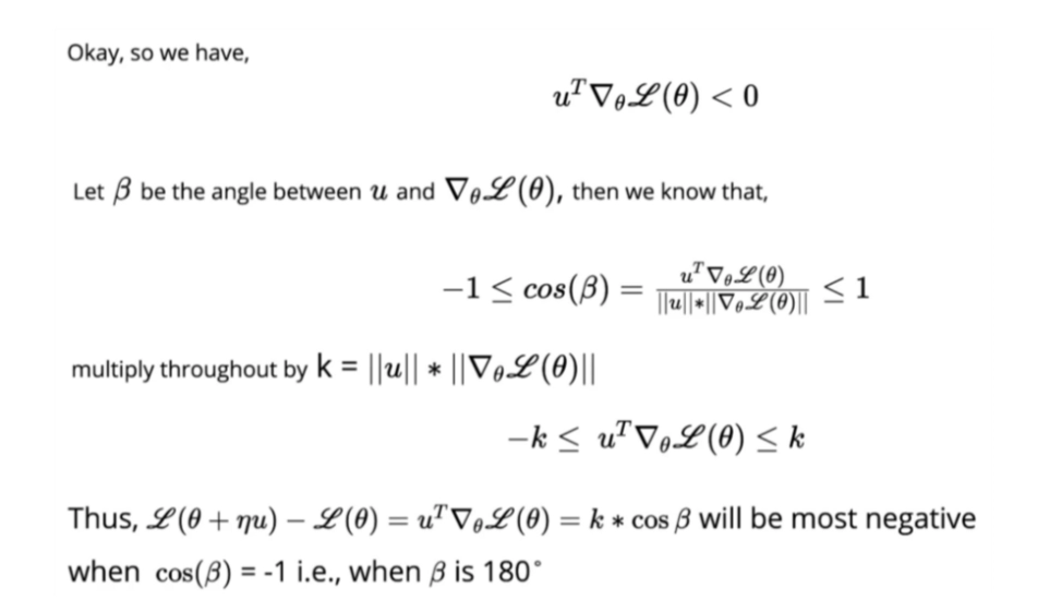
To solve the above equation, let’s apply a bit of linear algebra. As we know, the cosine angle between two vectors is cos(θ), ranging from -1 to 1.

Img src

 

Since the angle is equal to 180⁰, the direction of change vector uᵀ we choose should be opposite to the gradient vector.

 

Thus we can deduce the following results:

• The direction of the change vector that we intend to move should be in the opposite direction concerning the gradient(180 degrees).

 

So the last question with the learning algorithm is how to compute the partial derivatives for w and b?

Computing Partial Derivatives

Let us suppose we have to fit only one data point into the sigmoid neuron, so the loss function for one point can be written as,

 

 

Let us now derive the derivatives of the function:

Img src

 

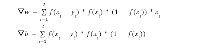
So the final equation is marked red above; in the case of two data points, the equation changes to:

 

Evaluation

With the help of the actual output and the predicted output, we can find the accuracy of the regression model by using RMSE(Root Mean Squared Error). While in the case of the classification model, we can evaluate the accuracy by :

 

accuracy=(total correct predictions)/(total number of predictions).

Implementation

Now moving into the implementation part,

X = [1.4,2.5] Y = [0.6,0.9] import numpy as np import matplotlib.pyplot as plt from matplotlib import cm from mpl_toolkits.mplot3d import Axes3D %matplotlib inline w_values = [] b_values = [] loss_values = [] def f(w,b,x):     return 1. / (1. + np.exp(-(w*x)+b))    def error(w,b):   err = 0.0   for x,y in zip(X,Y):     fx = f(w,b,x)     err += 0.5*(fx-y)**2   return(err) def grad_w(w,b, x, y):     y_pred = f(w,b,x)     return (y_pred - y) * y_pred * (1 - y_pred) * x def grad_b(w,b, x, y):     y_pred = f(w,b,x)     return (y_pred - y) * y_pred * (1 - y_pred) def gradient_descent():   w,b,eta = 0, -8, 1.0   for i in range(1000):       dw, db = 0, 0       for x, y in zip(X, Y):           dw += grad_w(w,b,x, y)           db += grad_b(w,b,x, y)       w -= eta*dw       b -= eta*db       w_values.append(w)       b_values.append(b)       loss_values.append(error(w,b)) gradient_descent()

 

Frequently Asked Questions

1. What is the difference between Sigmoid and ReLU?
   Relu is more computationally efficient than Sigmoid functions since Relu finds the max(0,x) and does not perform expensive exponential operations as in the case of Sigmoids.
    
2. What are the properties of the sigmoid neuron?
   In the sigmoid neuron, a slight change in the input causes a small change in the output instead of the stepped work–many functions characteristic of an "S" shaped curve known as sigmoid functions.
    
3. What are the limitations of the sigmoid neuron?
   The two significant limitations with sigmoid activation functions are: Sigmoid saturation and kill gradients: The output of sigmoid saturates (i.e., the curve becomes parallel to the x-axis) for a significant positive or negative number. Thus, the gradient at these regions is almost zero.

Key Takeaways

Let us brief the article.

 

Firstly, we saw the limitation of the perceptron neuron that led to the discovery of the sigmoid neuron. Furthermore, we saw how sigmoid neurons overcome the limits of the Perceptron. We saw the building blocks to develop a sigmoid neuron, then moving forward, we saw the in-depth intuition of the learning algorithm with the help of the Taylor series, linear algebra, and partial derivatives. And at last, we saw the implementation of the learning algorithm. 

 

That's the end of the article. Stay updated for more exciting articles like these.

Recommended Reading:

• Introduction to Machine Learning

Happy Learning Ninjas!