Example
Here’s a basic implementation of Simulated Annealing in Python:
Python
import math
import random
# Objective Function
def objective_function(x):
return x**2 - 4*x + 4
# Simulated Annealing Algorithm
def simulated_annealing():
current_solution = random.uniform(-10, 10) # Start with a random solution
current_value = objective_function(current_solution)
best_solution = current_solution
best_value = current_value
temperature = 100.0 # Initial temperature
cooling_rate = 0.95 # Rate at which the temperature decreases
while temperature > 1e-3:
new_solution = current_solution + random.uniform(-1, 1)
new_value = objective_function(new_solution)
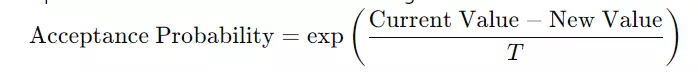
if new_value < best_value or random.uniform(0, 1) < math.exp((current_value - new_value) / temperature):
current_solution = new_solution
current_value = new_value
if new_value < best_value:
best_solution = new_solution
best_value = new_value
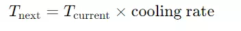
temperature *= cooling_rate
return best_solution, best_value
# Run the algorithm
best_solution, best_value = simulated_annealing()
print(f"Best Solution: {best_solution}")
print(f"Best Value: {best_value}")

You can also try this code with Online Python Compiler
Output
Best Solution: 1.025
Best Value: 0.050
Explanation of the Output
Best Solution:
This represents the value of xxx where the algorithm found the optimal or near-optimal result. In this example, Best Solution: 1.025 means that the best value for xxx found by the algorithm is approximately 1.025.
Best Value:
This is the minimum value of the objective function at the best solution. For the function f(x)=x2−4x+4f(x) = x^2 - 4x + 4f(x)=x2−4x+4, the Best Value: 0.050 indicates the function’s minimum value at x=1.025x = 1.025x=1.025.
How is Simulated Annealing Used in Artificial Intelligence?
- Scheduling Problems: Simulated Annealing helps assign timeslots and resources to tasks to minimize total duration and cost. For example, it can organize employee shifts or production schedules efficiently.
- Routing Problems: It solves routing issues, like the traveling salesman problem. The goal is to find the shortest route that visits a set of locations and returns to the start, which helps in optimizing logistics and deliveries.
- Machine Learning: In neural network training, Simulated Annealing adjusts hyperparameters, such as learning rates or network structure, to improve model performance.
- Game Playing: Simulated Annealing aids game AI in making strategic decisions. It evaluates different moves based on a scoring system to choose the best action.
Why is Simulated Annealing Used in Artificial Intelligence?
- Flexibility and Generality:Simulated Annealing can be applied to nearly any optimization problem, regardless of the problem's domain.
- Global Search Capability:Unlike gradient-based methods that may get stuck in local minima, Simulated Annealing has a better chance of finding the global minimum.
- Simple Implementation:The algorithm is easy to implement, often requiring just a few lines of code to tackle various problems.
- Adaptability:Simulated Annealing can handle different constraints and complex objective functions, even if they are non-differentiable or discontinuous.
Applications of Simulated Annealing in AI
- Traveling Salesman Problem (TSP): Finding the shortest possible route that visits a set of cities and returns to the origin city.
- Job Scheduling: Optimizing job schedules to minimize total completion time or maximize resource utilization.
- Machine Learning: Tuning hyperparameters of machine learning models to achieve better performance.
- Layout Optimization: Designing efficient layouts for circuit boards, wireless networks, or production processes.
Key Features of Simulated Annealing in AI
- Global Optimization:The algorithm aims to avoid local minima and seek a global optimum.
- Probabilistic Acceptance:It accepts worse solutions with a certain probability to escape local optima.
- Cooling Schedule:The temperature parameter decreases over time, which controls the likelihood of accepting worse solutions.
Disadvantages of Using Simulated Annealing in AI
- Computationally Expensive: Cooling and exploring many solutions can be resource-intensive, especially for large or complex problems.
- Sensitive to Parameters: The algorithm’s performance depends on the cooling schedule and initial settings. Poor choices can result in slow convergence and suboptimal solutions.
- Randomness: The algorithm’s stochastic nature can lead to inconsistent results. Different runs might produce varied outcomes, which can be problematic for applications requiring high reliability.
- Slow Convergence: As the temperature decreases, the chance of accepting worse solutions reduces, which can slow convergence, particularly close to the global optimum.
Frequently Asked Questions
What is Simulated Annealing in AI?
Simulated Annealing is an optimization technique inspired by the annealing process in metallurgy. It searches for the best or near-best solution by probabilistically accepting worse solutions to avoid getting stuck in local optima.
What are the main parameters in Simulated Annealing?
The main parameters include the initial temperature, cooling rate, and stopping criteria. The temperature controls the probability of accepting worse solutions, and the cooling rate determines how quickly the temperature decreases.
What are the advantages of Simulated Annealing?
Simulated Annealing can escape local minima and approach a global optimum. It is versatile and can be applied to various optimization problems.
Conclusion
Simulated Annealing in AI is a strong optimization method used to tackle complex problems. It works by exploring different solutions and refining them to avoid local minima and find near-optimal solutions. This makes it useful for many tasks. By understanding how it works and using it properly, you can solve various optimization challenges in AI effectively.
You can also check out our other blogs on Code360.


 9+ registered

