Do you think IIT Guwahati certified course can help you in your career?
Introduction
Smoothing is often used to reduce noise within an image or produce a less pixelated image. Image smoothing is a key image enhancement technology that can remove noise within the images. So, it is a mandatory functional module in various image-processing software.
Image smoothing is a method of improving the quality of images. Image quality is an important factor for human vision. The image usually has noise that is not easily eliminated in image processing. The quality of the image is affected by the presence of noise. Many methods are there for removing noise from images. Many image processing algorithms can't work well in a noisy environment, so an image filter is adopted as a preprocessing module. However, the capability of conventional filters based on pure numerical computation is broken down rapidly when they are put in a heavily noisy environment.
Smoothing filters are used in noise reduction and blurring.
Blurring is used in preprocessing tasks, such as the removal of small details from an image before (large) object extraction.
Smoothing is used to produce less pixelated images.
In this article, we will see the following four topics:
Simple average blurring
Gaussian Blurring
Median filtering
Bilateral filtering
Simple Average Blurring
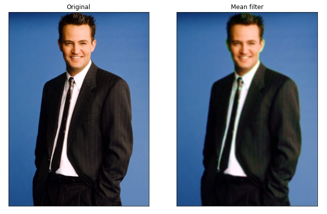
Simple average blurring can also be termed mean filtering. The mean filter is used to remove noise from the image and helps in making the image blur. It includes determining the mean of the pixel values within an n x n kernel. The mean then replaces the pixel intensity of the center element. This helps in eliminating some of the noise in the image and smoothening the edges of the image. We can use the blur function from the open-cv library to apply the mean filter.
First, we need to convert the image from RGB to HSV (hue saturation and value) because the dimensions of RGB depend on each other, whereas the three dimensions in HSV are independent of each other (this allows us to apply filters to each of the three dimensions separately).
Properties of Average Blurring
The amount of intensity variation between two neighboring pixels is reduced.
The Average blurring is a low-pass uniform filter.
All the elements of the kernel must be the same.
Method to replace each pixel with mean.
Consider an image of 5 x 5 pixels as shown below and a kernel of size 3 x 3. If we want to replace the middle pixel i.e. (3,3) then take the sum of all the neighboring pixels including itself and divide it by kernel size i.e., (65 + 45 + 32 + 25 + 67 + 11 + 23 + 78 + 32)/9 = 41. So 67 will be replaced by 41. Similarly, we will replace all the remaining pixels.
12
23
4
32
44
32
65
45
32
42
21
25
67
11
23
45
23
78
32
23
45
34
89
66
21
Code for Average Blurring (Mean Filter)
# importing libraries
import numpy as np
import cv2
from matplotlib import pyplot as plt
%matplotlib inline
from PIL import Image
from PIL import ImageFilter
You can also try this code with Online Python Compiler
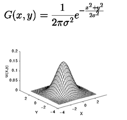
The Gaussian filter is the same as the mean filter; however, it involves a weighted average of the surrounding pixels and has sigma as a parameter. The kernel used in Gaussian blurring represents a discrete approximation of a Gaussian distribution. The Gaussian filter helps in preserving the edges of the image. The Open-CV library provides a function called the "GaussianBlur" that helps in implementing a Gaussian filter. The GaussianBlur function allows you to specify the shape of the kernel and standard deviation for the x and y directions separately. If only one sigma value is specified, it is considered the sigma value for both the x and y directions.
The formula and the graph for the Gaussian distribution of a kernel are
Properties of Gaussian Blurring
The Gaussian blurring is a non-uniform low-pass filter.
The coefficients of the kernel decrease as the distance from the center increases.
Pixels at the center have a higher weight than the pixels at the periphery.
The image's brightness may not be preserved after applying a Gaussian filter.
The kernel is rotationally symmetric.
Method of calculating Gaussian Blurring
Let us consider the image of size 5 x 5 pixels and a kernel of size 3 x 3 pixels.
Image
12
23
4
32
44
32
65
45
32
42
21
25
67
11
23
45
23
78
32
23
45
34
89
66
21
Kernel
1
2
1
2
4
2
1
2
1
If we want to replace the (3, 3) pixel of the image we have to calculate a weighted average of the pixel.
Weighted average =
(1/16)(65x1 + 45 x 2 + 32 x 1 + 25 x 2 + 67 x 4 + 11 x 2 + 23 x 1 + 78 x 2 + 32 x 1)
Similarly, update all the pixels of the image.
Code for Gaussian Blurring
Importing libraries
import numpy as np
import cv2
from matplotlib import pyplot as plt
%matplotlib inline
from PIL import Image
from PIL import ImageFilter
You can also try this code with Online Python Compiler
The median filter calculates the median of the pixel intensities surrounded by the center pixel in a n x n kernel. The intensity of the center pixel is then replaced with a median. It helps in removing salt and pepper noise from the image. This preserves the edges of an image, but it does not handle speckle noise. The Open-CV library provides a "medianBlur" function that helps in implementing the median blur filter.
Properties of Median Filtering
Median filtering is a non-linear digital filtering technique.
It helps to preserve edges while removing noise from the images.
It is used in removing salt and pepper noise.
Method of calculating Gaussian Blurring
Let us consider the image of size 5 x 5 pixels, and a kernel of size 3 x 3 pixels.
Image
12
23
4
32
44
32
65
45
32
42
21
25
67
11
23
45
23
78
32
23
45
34
89
66
21
If we want to replace the pixel of the image at positions (3, 3) we have to calculate the median of all the nearest pixels.
The median of (65, 45, 32, 25, 67, 11, 23, 78, 32) is 32 so, the pixel at position 3,3 will be replaced with 32
Similarly, update all the pixels of the image.
Code for Median Filtering
Importing libraries
import numpy as np
import cv2
from matplotlib import pyplot as plt
%matplotlib inline
from PIL import Image
from PIL import ImageFilter
You can also try this code with Online Python Compiler
A bilateral filter is a non-linear, edge-preserving, noise-reducing filter used for smoothing images. The intensity of each pixel is replaced with a weighted mean of intensity values from nearby pixels. The weights of the filter are based on a Gaussian distribution. Crucially, the weights depend not only on the Euclidean distance of pixels but also on the radiometric differences (e.g., range differences, such as color intensity, depth distance, etc.). This filtering preserves sharp edges.
The following image shows how to preserve edges by spatial and color(intensity) weights.
Two pixels are close to each other in bilateral filtering if they occupy neighboring spatial positions and exhibit some photometric range similarity.
Bilateral filtering takes the Gaussian filter in space and considers another Gaussian filter that is a function of pixel difference. For this reason, bilateral filters preserve edges as the pixel at the edges have large intensity variation.
The formula for Bilateral filtering
Bilateral filtering is represented by the symbol BF.
Here Wp is the normalization factor. The value of Wp is given below.
In the above equations, Gσs is a spatial Gaussian that decreases the influence of distant pixels. Gσr is a range Gaussian that decreases the influence of pixels q with an intensity value different from Ip. σs is the space parameter it represents the spatial extent of the kernel size of the considered neighborhood and σr is the range parameter that represents the minimum amplitude of an edge. Both the parameters will measure the amount of filtering for image I.
Code for Bilateral Filtering
Importing libraries
import numpy as np
import cv2
from matplotlib import pyplot as plt
%matplotlib inline
from PIL import Image
from PIL import ImageFilter
You can also try this code with Online Python Compiler
What are the techniques used for image smoothing? Low pass filtering (aka smoothing) removes high spatial frequency noise from a digital image. The low-pass filters usually employ a moving window operator that affects one pixel of the image at a time.
What is image smoothing and sharping? Color image smoothing is part of preprocessing techniques intended for removing possible image perturbations without losing image information. Analogously, sharpening is a preprocessing technique that plays an important role in feature extraction in image processing.
How does a gaussian blur work? In a Gaussian blur, the pixels near the kernel's center are given more weight than those far away from the center. This averaging is done on a channel-by-channel basis, and the value of the pixel is replaced with the average channel value.
What is meant by Gaussian? being or having the shape of a normal curve or a normal distribution.
What is the difference between mean and median filtering? The median is a more robust average than the mean, so a single very unrepresentative pixel in a neighborhood will not significantly affect the median value.
Key Takeaways
In this article, we have studied the following topics:
Uses of image smoothing
Mean Blurring
Gaussian Blurring
Median Filtering
Bilateral Filtering
Want to learn more about Machine Learning? Here is an excellent course that can guide you in learning.
Happy Coding!
Live masterclass
Prompt Engineering: Must-have GenAI Skill for 30L+ Roles at Amazon
by Anubhav Sinha
16 Jul, 2026
12:30 PM
Using Netflix Data to Master Power BI
by Ashwin Goyal
13 Jul, 2026
12:30 PM
Top GenAI Skills to crack 30L+ CTC at Amazon & Google
by Sumit Shukla
14 Jul, 2026
11:30 AM
JioHotstar Sports Analytics using IPL Dataset
by Prerita Agarwal
15 Jul, 2026
12:30 PM
Prompt Engineering: Must-have GenAI Skill for 30L+ Roles at Amazon


 9+ registered

