


📜Softmax Function📜
Suppose there's a case where we divide our neural network into two categories: boy and girl.

How do we know that the two classes coordinate their probabilities to sum up to one? Well, the answer is they don't blend these results. The reason that the results have this coherence is that we use the softmax function.
The softmax function, also known as softargmax or normalized exponential function, generalizes the logistic function to multiple outputs. We use the softmax function in multinomial logistic regression and the last activation function in a neural network to normalize the network's output to a probability distribution over predicted output classes.

The softmax function takes an input vector of K real numbers. It normalizes it into a probability distribution consisting of K probabilities proportional to the exponentials of the input numbers. Before applying softmax, some vector components could be negative or greater than one and might not sum to one. But after using the softmax function, each component will be in the interval (0,1), and the components will sum up to one so that they can be interpreted as probabilities.
The softmax function is represented as
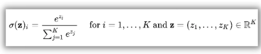
In simple words, the softmax function applies the standard exponential function to each element of the input vector z. It normalizes these values by dividing them by the sum of all these exponentials. This normalization ensures that the sum of the components of the output vector is one.
🧑💻Implementation🧑💻
import numpy as np
a = [1,5,6,4,2,2.6,6]
vector=np.exp(a) / np.sum(np.exp(a))
👉Output:
array([0.00263032, 0.14361082, 0.39037468, 0.05283147, 0.00714996,
       0.01302808, 0.39037468])
Also Read, Resnet 50 Architecture
📜Cross-Entropy📜
If we remember the artificial neural networks section material, we had the mean squared error function. We use this function to assess the performance of our network, and by working to minimize this mean squared error, we are practically optimizing the network. The mean squared error function can be used with convolutional neural networks. Still, an even better option would be applying the cross-entropy function after you had entered the softmax function.

We relate cross-entropy loss closely to the softmax function since it's practically only used with networks with a softmax layer at the output. We extensively use cross-entropy loss in multi-class classification tasks, where each sample belongs to one of the C classes. The label assigned to each sample consists of a single integer value between 0 and C -1. A one-hot encoded vector of size can represent the label C. We label the correct class as one and zero everywhere else.
Cross-entropy takes as input two discrete probability distributions (simply vectors whose elements lie between zero to one and add up to one) and outputs a single real-valued (!) number representing the similarity of both probability distributions.
It is defined as,

The larger the value of cross-entropy, the less similar the two probability distributions are. When cross-entropy is used as a loss function in a multi-class classification task, y is fed with the one-hot encoded label. The symbols represent the probabilities generated by the softmax layer.
The above equation shows that we take logarithms of probabilities generated by the softmax layer, so we won't take the logarithm of zero as softmax will never produce zero values. We force the predicted probabilities to gradually resemble the accurate one-hot encoded vectors by minimizing the loss during training.
🧑💻Implementation🧑💻
👉Importing Libraries
import numpy as np
import matplotlib.pyplot as plt
👉Cross-Entropy function
def cross_entropy_loss(yHat, y):
    if y == 1:
      return -np.log(yHat)
    else:
      return -np.log(1 - yHat)
👉Sigmoid Function
def sigmoid(z):
    return 1.0 / (1.0 + np.exp(-z))
👉Dataset
z = np.arange(-5, 5, 0.2)
# Calculating the probability value
h_z = sigmoid(z)
👉Loss when y=1
# Value of cost function when y = 1
cost_1 = cross_entropy_loss(h_z, 1)
👉Loss when y=0
# Value of cost function when y = 0
cost_0 = cross_entropy_loss(h_z, 0)
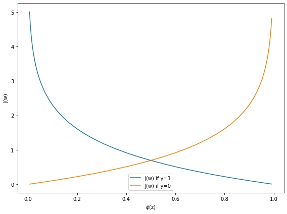
👉Plotting
fig, ax = plt.subplots(figsize=(8,6))
plt.plot(h_z, cost_1, label='J(w) if y=1')
plt.plot(h_z, cost_0, label='J(w) if y=0')
plt.xlabel('$\phi$(z)')
plt.ylabel('J(w)')
plt.legend(loc='best')
plt.tight_layout()
plt.show()
👉Output


 9+ registered

