Introduction
When dealing with sequential data, one must prefer recurrent neural networks over any other neural networks because RNN maintains internal memory so that it can store the data of previous input data. But there is a drawback to using an RNN because it causes a vanishing gradient problem in simple RNN. For this reason, an updated RNN known as LSTM is widely used.
In the following article, we will see how RNN causes vanishing gradient problems and also will see how this problem can be solved using LSTM.
Vanishing Gradient Problem
RNNs are plagued by the problem of vanishing gradients, which makes learning large data sequences difficult. The gradients contain information utilized in the RNN parameter update, and as the gradient shrinks, the parameter updates become minor, implying that no meaningful learning occurs.
Now let us see the proof that RNN causes a vanishing gradient problem.
Also Read, Resnet 50 Architecture
RNN and Vanishing Gradient Problem
Let us have a look at the basic architecture of the recurrent neural network. The image below is an RNN.
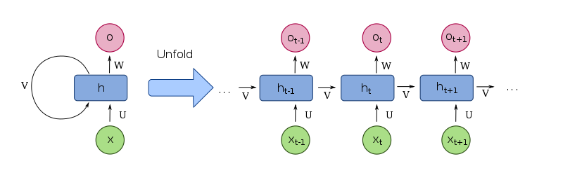
The neural network has an input sequence of [x(1), x(2),…, x(k)]; at a time step t, we provide an input of x(t). Past information and learned knowledge are encoded in the neural network as vectors [c(1), c(2),…, c(k-1)], at time step t, the neural network has a state vector of c(t-1). The state vector c(t-1) and the input vector x(t) these two vectors are attached to make a complete input vector at time step t, i.e., [c(t-1), x(t)].
The two-weight matrices: Wrec and Win, of the neural network, are connecting to two parts of the input vector c(t-1) and x(t), to the hidden layer. We ignore the bias vectors in our calculations and write W = [Wrec, Win] instead.
In the hidden layer, the sigmoid function is utilized as the activation function.
At the last time step, the network produces a single vector (RNNs can output a vector at each time step, but we'll use this simplified model).
Backpropagation Through Time in RNNs
We compute the prediction error E(k) and utilize the Back Propagation Through Time approach to computing the gradient after the RNN outputs the prediction vector h(k).
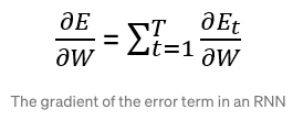
We use the gradient to update the weights of the models in the following way.

Now we apply the gradient descent algorithm to the neural network and continue the learning process.
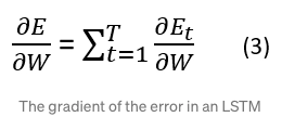
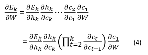
If the learning process has total T time steps, then the gradient of the error on the kth time step will be:
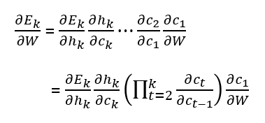
As we can write W = [Wrec, Win], therefore c(t) can be written as:

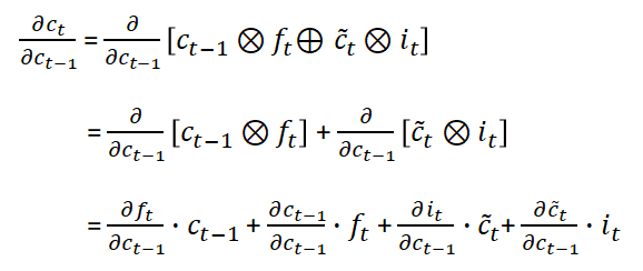
Computing the derivative of c(t):

Now insert the derivative of c(t) in the gradient of the error in the kth step’s equation.

When k is big, the last statement tends to vanish because the derivative of the tanh activation function is lower than 1.
The exploding gradient problem can also occur when the weights Wrec are strong enough to override the smaller tanh derivative, causing the product of derivatives to explode.
We have:

At some time step k:

Due to this, our complete gradient will vanish.
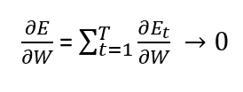
And the neural network will be updated in the following way:

So the weights (W) will not have any significant change, and hence learning of neural networks will have no progress.


