Spam/Ham Classification using Naive Bayes

Spam/Ham Classification using Naive Bayes

Understanding the dataset 

For spam/ham classification, here we have taken our training dataset from Kaggle. The dataset contains 5000+ text messages samples categorized under the category of spam/ham depending on the content of the messages. 

Step 1: Import all the required libraries

import numpy as np
import pandas as pd
import matplotlib.pyplot as plt
import seaborn as sns

 

Step 2: Import the data and print the head to have a fundamental outlook of the data. In this case, we are using the.csv file from Kaggle named spam.csv. 

df_sms = pd.read_csv('spam.csv',encoding='latin-1')
df_sms.head()

 

Output:

 

Data Cleaning

Step 3: As we can see, we have some unwanted columns. Let’s drop them and have a more optimized table of the dataset. 

df_sms = df_sms.drop(["Unnamed: 2", "Unnamed: 3", "Unnamed: 4"], axis=1)
df_sms = df_sms.rename(columns={"v1":"label", "v2":"sms"})
df_sms.head()

 

Output: 

Step 4: Print total values of spam and ham in the given dataset to the in-depth idea of our given dataset. 

df_sms.label.value_counts()

 

Output:

ham     4825
spam     747
Name: label, dtype: int64

 

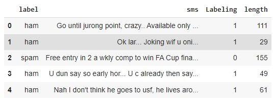
Step 5: Since we want our answers in binary and it is easy for computation, let's convert our data into 0 and 1 for spam and ham. 

df_sms['Labeling']= df_sms['label'].map({'ham': 1, 'spam':0})
df_sms.head()

 

Output:

Step 6: Let’s find the length of every spam/ham message to help categorize them better. 

df_sms['length'] = df_sms['sms'].apply(len)
df_sms.head()

 

Output: 

 

Step 7: Let’s visualize the data of length using a histogram. 

import matplotlib.pyplot as plt
import seaborn as sns

%matplotlib inline
df_sms['length'].plot(bins=50, kind='hist')

 

Output: 

Step 7: Using a histogram, let’s also visualize the segregated length of spam/ham messaged in our given dataset. 

df_sms.hist(column='length', by='label', bins=50,figsize=(10,4))

 

Output: 

Splitting the dataset in train and test 

Step 8: Let’s train the model using the sklearn library. 

X = df_sms['sms']
Y = df_sms['Labeling']
from sklearn.model_selection import train_test_split as tt
X_train, X_test, Y_train, Y_test = tt(X, Y,test_size=0.2, random_state=100)

 

Step 9: Let’s find the x test and train shape for the split data. 

X_train.shape

 

Output: 

(4457,)

 

X_test.shape

 

Output:

(1115,)

 

Exclude Stop Words

Step 10: Words that are not in our English dictionaries should be excluded from our data as they cause unnecessary errors. For this, we use the sklearn vector feature.

from sklearn.feature_extraction.text import CountVectorizer
vector = CountVectorizer(stop_words ='english')
vector.fit(X_train)

 

Step 11: Print the frequency of the words used. 

vector.vocabulary_

 

Output:

{'clearing': 1819, 'cars': 1642’ 'meant': 4323, 'calculation': 1577, 'units': 6960, 'expensive': 2677, 'started': 6274, 'practicing': 5214, 'accent': 784, 'important': 3549, 'decided': 2183, '4years': 539, 'dental': 2226, 'nmde': 4684, 'exam': 2656, 'idk': 3516, 'sitting': 6023, 'shop': 5939, 'parking': 4954, 'lot': 4124, 'bawling': 1240, 'feel': 2759, ...}

 

Step 12: Let’s train the model with the final vector inputs and proceed to prediction.

X_train_transformed =vector.transform(X_train)
X_test_transformed =vector.transform(X_test)

 

Building the Final Model sing Naive Bayes

Step 13: We import the multinomial naive Bayes libraries from sklearn 

from sklearn.naive_bayes import MultinomialNB
model = MultinomialNB()
model.fit(X_train_transformed,Y_train)
y_pred = model.predict(X_test_transformed)
y_pred_prob = model.predict_proba(X_test_transformed)

 

Performing the Predictions 

Step 14: To help the model predict, we import the confusion matrix, accuracy score, precision score, recall score, and f1 score. 

from sklearn.metrics import confusion_matrix,accuracy_score,precision_score,recall_score,f1_score
print(confusion_matrix(Y_test,y_pred))
print()
print(accuracy_score(Y_test,y_pred))

 

Output:

[[135  10]
 [  9 961]]

0.9829596412556054

 

Step 15: Print all the predictions made

print(precision_score(Y_test,y_pred))
print()
print(recall_score(Y_test,y_pred))
print()
print(f1_score(Y_test,y_pred))
print()

 

Output:

0.9897013388259527

0.9907216494845361

0.9902112313240599

 

ROC curve

Step 16: Import the ROC curve feature from sklearn to find true and false positives. 

from sklearn.metrics import roc_curve, auc

false_positive_rate, true_positive_rate, thresholds = roc_curve(Y_test, y_pred_prob[:,1])
roc_auc = auc(false_positive_rate, true_positive_rate)
print(roc_auc)

 

Output:

0.9866619267685744

 

print(false_positive_rate)
print()
print(true_positive_rate)
print()
print(thresholds)

 

Output:

[0.         0.         0.         0.         0.         0.
 0.         0.         0.         0.         0.         0.
 0.         0.00689655 0.00689655 0.00689655 0.00689655 0.00689655
 0.00689655 0.00689655 0.00689655 0.00689655 0.00689655 0.00689655
 0.00689655 0.00689655 0.00689655 0.00689655 0.00689655 0.00689655
 0.00689655 0.0137931  0.0137931  0.0137931  0.0137931  0.0137931
 0.0137931  0.0137931  0.0137931  0.0137931  0.0137931  0.02068966
 0.02068966 0.02068966 0.02068966 0.02068966 0.02068966 0.02068966
 0.02068966 0.02068966 0.02068966 0.02068966 0.02068966 0.02068966
 0.02068966 0.02068966 0.02758621 0.02758621 0.02758621 0.02758621
 0.02758621 0.02758621 0.02758621 0.02758621 0.02758621 0.02758621
 0.02758621 0.02758621 0.02758621 0.02758621 0.03448276 0.03448276
 0.03448276 0.03448276 0.03448276 0.03448276 0.03448276 0.03448276
 0.03448276 0.03448276 0.03448276 0.04137931 0.04137931 0.04827586
 0.04827586 0.05517241 0.05517241 0.06206897 0.06206897 0.06896552
 0.06896552 0.06896552 0.06896552 0.08275862 0.08275862 0.09655172
 0.09655172 0.10344828 0.10344828 0.11034483 0.11034483 0.29655172
 0.31034483 0.54482759 0.55862069 0.69655172 0.71034483 0.8
 0.82758621 0.84827586 0.86206897 0.88275862 0.89655172 0.9862069
 1.        ] 

 

Step 18: Find the FPR. Threshold and TPR for the data. 

df = pd.DataFrame({'Threshold': thresholds, 
              'TPR': true_positive_rate, 
              'FPR':false_positive_rate
             })
df.head()

 

Output:

 

Step 19: Plot the ROC curve of the dataset. 

%matplotlib inline  
plt.ylabel('True Positive Rate')
plt.xlabel('False Positive Rate')
plt.title('ROC')
plt.plot(false_positive_rate, true_positive_rate)

 

Output:

Frequently Asked Questions

Q1. Can we use Bernoulli Naive Bayes classification for spam/ham?

Ans: Yes, we can use gaussian naive Bayes classification. Instead of importing the multinomialNB, we will import the BernoulliNB.

from sklearn.naive_bayes import BernoulliNB
modelB = BernoulliNB()

 

Q2. When is the best time to use naive Bayes classification? 

Ans: When the independence requirement is met, a Naive Bayes classifier outperforms alternative models such as logistic regression and requires less training data. When compared to numerical variables, it performs well with categorical input variables. 

 

Q3.Does naive Bayes come under supervised or unsupervised learning? 

Ans: Naive Bayes classification comes under supervised learning. It is supervised because naive Bayes classifiers are trained on labeled data, i.e., data pre-categorized into the classes accessible for classification.

Key Takeaways

Spam messages can be a real headache and can cause a lot of inconveniences to the users. In this article, we have discussed the application of spam/ham classification using naive Bayes from scratch. We have first discussed naive Bayes to know how Naive Bayes works; later on, we went with the classification of spam/ham using our code in python. 

To read more such interesting real-world implementation of concepts, read our blogs at the coding ninjas’ website.