Table of contents
1.
Introduction
2.
Support Vector Machine and its basic intuition
3.
Hyperparameters of Support Vector Machine
3.1.
1. Kernel Function
3.2.
2. C (Regularization)
3.3.
3. Gamma
4.
GridSearchCV
5.
Code: SVM hyperparameter tuning using GridSearchCV
6.
Frequently Asked Questions
7.
Key Takeaways
Last Updated: Jun 26, 2024

SVM Hyperparameter Tuning using GridSearchCV

Author Toohina Barua
0 upvote
Career growth poll
Do you think IIT Guwahati certified course can help you in your career?

Introduction

Do you want to know about the machine learning algorithm that can be used in both face detection and Bioinformatics? Well, you have come to the right place! In this article, we will talk about Support Vector Machines.  Not only this, but we are also going to see how we can make our model highly accurate by changing its hyperparameters. However, finding the optimal values for these hyperparameters can be cumbersome and time-consuming if you do it manually. So, what should we do to make this task easier? We use GridSearchCV! Let’s discuss SVM, SVM hyperparameters, and their tuning with GridSearchCV both theoretically and practically!

Support Vector Machine and its basic intuition

Support vector machines fall under supervised machine learning techniques that are mainly used for classification problems. You can use it for regression problems too. 

The basic idea behind the Support vector machine is that it takes data of relatively low dimension and converts it into higher dimensional data. Then it classifies the data into different categories by separating the data using a Hyperplane.  

Let us understand the basic intuition behind a support vector machine using an example:

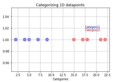
Let us imagine that we have a training dataset. The training data have been divided into category one (blue) and category two (red).

If we pass our training data through our model, it will set a decision boundary/threshold in the center of the last blue and the first red observations. The threshold is shown with the green line.

Note: The decision boundary, in this case, is a point, but it has been represented with a line to be visible properly without leading to confusion. 


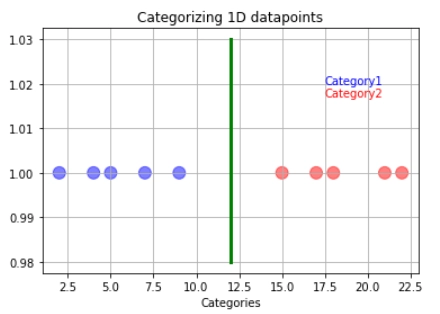
So if new data comes, we can easily classify it into either category one or category two depending on which side of the line they are.

But what happens if the training data has outliers? Suppose our model follows the hard and fast rule of making a boundary directly at the middle of the last category one and first category two observations. 

In that case, this may lead to wrong predictions regarding the testing data. In this example, the orange data point represents the new data.

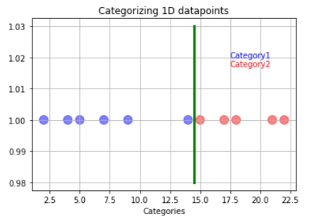
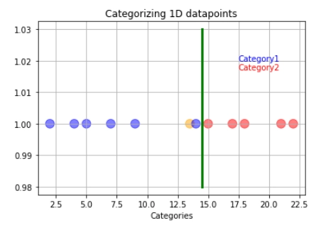
The orange data will get classified as blue instead of red even though it is closer to the red data point. So how do we overcome the problem of outliers? It is simple: We just have to allow misclassifications!

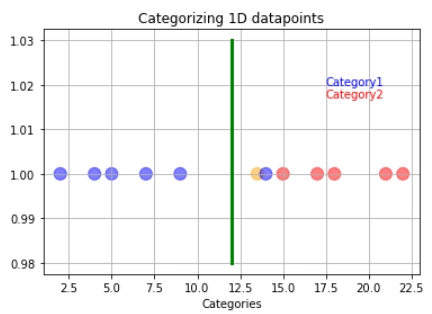
We allow the outlier to be misclassified as red data to have a better decision boundary. When we allow misclassification within the margin, the margin is called a soft margin

In the case above, what we are using is a support vector classifier. We are using the support vector classifier to find the suitable decision boundary by allowing misclassifications. 


Source


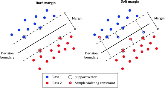
Allowing misclassification is a part bias-variance trade-off as we put some of the training data into the wrong category so that our model works well on testing data.

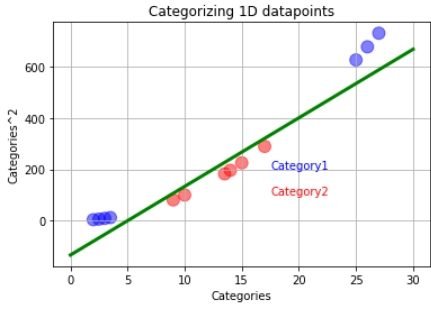
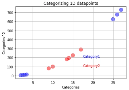
But what if our training data looks like below:

In a case like this, we will use the support vector machines. The support vector machine first converts the lower dimension training data into higher dimensional data. In this case, from one dimension, the data gets converted into two-dimension. How is this done? The square of the data becomes the y axis.

After this, we find the suitable decision boundary using the support vector classifier. In this case, our decision boundary becomes a two-dimensional hyperplane.


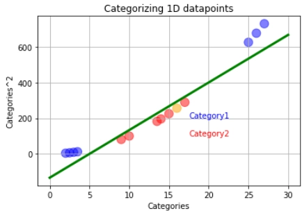
If new data comes, the support vector machine will square it and classify it depending on which side of the hyperplane it is. The orange data represents the latest data. It will be classified into the red category.

The code for all the graphs is given below:

#imports
import pandas as pd
import numpy as np
from sklearn import datasets
from sklearn.model_selection import train_test_split
from sklearn.svm import SVC  
from sklearn.metrics import classification_report, confusion_matrix 
from sklearn.model_selection import GridSearchCV
import matplotlib.pyplot as plt
import seaborn as sns

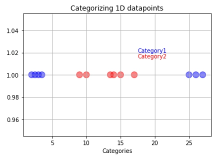
#So what should we do to make our classifier not sensitive to outliers?
#WE SHOULD ALLOW MISSCLASSIFATION
x7=[2,4,5,7,9,13.5,14,15,17,18,21,22]
y7=np.ones(12)
size=np.ones(12)*120
colors=['b','b','b','b','b','orange','b','r','r','r','r','r']
plt.title("Categorizing 1D datapoints")
plt.xlabel("Categories")
plt.text(x=17.5, y=1.02, s="Category1",color='b')
plt.text(x=17.5, y=1.0170, s="Category2",color='r')
plt.scatter(x7,y7,s=size,c=colors,alpha=0.5)


#making the support vector classifier threshold with soft margin
x8=np.ones(4)*(((15-9)/2)+9)
y8=[0.98,1,1.02,1.03]
plt.plot(x8,y8,c='green',linewidth=3)
plt.grid()
print(plt.show())

#category1=[2,4,5,7,18,21,22] 
#category2=[9,10,14,13.5,15,17] 
#16 is the new data
x12=np.array([2,2.5,3,3.5,9,10,13.5,14,15,16,17,25,26,27])
y12=(x12)**2

size=np.ones(14)*120
colors=['b','b','b','b','r','r','r','r','r','orange','r','b','b','b']
plt.title("Categorizing 1D datapoints")
plt.xlabel("Categories")
plt.ylabel("Categories^2")
plt.text(x=17.5, y=200, s="Category1",color='b')
plt.text(x=17.5, y=100, s="Category2",color='r')
plt.scatter(x12,y12,s=size,c=colors,alpha=0.5)

#Finding the perfect support vector classifier
x13=np.array([0,5,10,15,20,25,30])
y13=((80/3)*x13)-(400/3) #calculated using simple line equation with two points
plt.plot(x13,y13,c='green',linewidth=3)
plt.grid()
print(plt.show())
You can also try this code with Online Python Compiler
Run Code

Hyperparameters of Support Vector Machine

Hyperparameters of any machine learning model are the parameters of the model. Changing these parameters will result in a different output every time. Tweaking these parameters may lead to the model giving better predictions or results. In the Support Vector Machine, the Hyperparameters are:

1. Kernel Function

Let’s revisit the above example:

The support vector machine transforms the one-dimensional data points into two by squaring them in the example above. The squaring is done by what’s called the Kernel Function. In this case, the polynomial kernel function of degree 2.

Apart from squaring the data, there are other ways to spread our data points across N-dimensional space. The kernel functions compute the correlation between the data points in higher dimensions to find the best support vector classifier. 

Some of the Kernel functions are:

  • Linear Kernel: It's the most basic sort of kernel, and it's usually one-dimensional. It is used for classification problems in which we can separate the data linearly. It is the fastest among all the kernel functions.
  • Polynomial Kernel: It is like a linear kernel but in higher dimensions. It has a parameter d, which is the degree of the polynomial.
  • Gaussian Radial Basis Function (RBF): It is used when the data is non-linear. 
  • Sigmoid Kernel: It is usually used in neural networks.


Source

Where,

x, xi =observations/ data points

coef = coefficient 

d= degree of polynomial

2. C (Regularization)

This parameter represents how much misclassification of the training data is allowed in the model. In the example we had discussed before, outliers can cause the model to have low bias and high variance. So if we change the Regularization parameter, we can increase or decrease the error in classifying training data by changing the width of the margin.

Source

3. Gamma

This parameter decides how much influence the data points at a certain distance from the hyperplane will have. If gamma is high, then nearby points will be considered. And if the gamma is low, far away points will have an influence too.


GridSearchCV

The Sklearn library has a function called GridSearchCV. It helps in determining the ideal hyperparameter values for a particular model by performing hyperparameter tuning. There is no way to know what the best values for hyperparameters are from the start itself. Manually adjusting hyperparameters would take a significant amount of time and resources. We use GridSearchCV to speed up the process.

GridSearchCV uses the Cross-Validation method to test all possible combinations of the values provided in the dictionary and analyzes the model for each one. As a result, we can get the accuracy for each combination of hyperparameters and choose the one that performs the best.

Code: SVM hyperparameter tuning using GridSearchCV

Let us see how to tune the hyperparameters of SVM using GridSearchCV and see what we can conclude from the data. We are going to work on the iris dataset.

#imports
import pandas as pd
import numpy as np
from sklearn import datasets
from sklearn.model_selection import train_test_split
from sklearn.svm import SVC  
from sklearn.metrics import classification_report, confusion_matrix 
from sklearn.model_selection import GridSearchCV
import matplotlib.pyplot as plt
import seaborn as sns

#loading iris data
iris = datasets.load_iris()
iris_data_df=pd.DataFrame(iris.data,columns=['sepal length (cm)',
  'sepal width (cm)',
  'petal length (cm)',
  'petal width (cm)'])
iris_target_df=pd.DataFrame(iris.target,columns=['class'])
iris_data_df.head(5)
You can also try this code with Online Python Compiler
Run Code


# 0='setosa', 1='versicolor',2='virginica'
iris_target_df.head(5) 
You can also try this code with Online Python Compiler
Run Code


x = iris.data #features
y = iris.target #target
x_train, x_test, y_train, y_test = train_test_split(x, y, random_state=42,test_size = 0.20) #splitting data into train test
You can also try this code with Online Python Compiler
Run Code


Let us compare the accuracy of all the kernel functions: 

#POLYNOMIAL KERNEL 
svc_polynomial = SVC(kernel='poly', degree=8, gamma="auto")
svc_polynomial.fit(x_train, y_train)# Make prediction
y_pred_polynomial = svc_polynomial.predict(x_test)# Evaluate our model
print("Evaluation: Polynomial kernel")
print(classification_report(y_test,y_pred_polynomial))
You can also try this code with Online Python Compiler
Run Code


#RADIAL KERNEL 
svc_RBF = SVC(kernel='rbf', gamma="auto")
svc_RBF.fit(x_train, y_train)# Make prediction
y_pred_RBF = svc_RBF.predict(x_test)# Evaluate our model
print("Evaluation: Radial kernel")
print(classification_report(y_test,y_pred_RBF))
You can also try this code with Online Python Compiler
Run Code


#SIGMOID KERNEL
svc_sig = SVC(kernel='sigmoid', gamma="auto")
svc_sig.fit(x_train, y_train)# Make prediction
y_pred_sig = svc_sig.predict(x_test)# Evaluate our model
print("Evaluation: Sigmoid kernel")
print(classification_report(y_test,y_pred_sig))
You can also try this code with Online Python Compiler
Run Code


#LINEAR KERNEL
svc_linear = SVC(kernel='linear', gamma="auto")
svc_linear.fit(x_train, y_train)# Make prediction
y_pred_linear = svc_linear.predict(x_test)# Evaluate our model
print("Evaluation: Linear kernel")
print(classification_report(y_test,y_pred_linear))
You can also try this code with Online Python Compiler
Run Code


The classification report shows that Radial and Linear kernels perform better than Polynomial of degree 8 and Sigmoid kernel functions. The Sigmoid kernel has the worst performance.

 Let us see if GridSearchCV can find the best combination of parameters (Kernel, C, gamma):

#Create a dictionary and fill out some parameters for kernels, C and gamma
grid_parameters = {'C': [0.1,1, 10, 100], 'gamma': [1,0.1,0.01,0.001],'kernel': ['poly','rbf', 'sigmoid','linear']}
grid = GridSearchCV(SVC(),grid_parameters,refit=True,verbose=2)
print(grid.fit(x_train,y_train))
You can also try this code with Online Python Compiler
Run Code


print(grid.best_estimator_)
You can also try this code with Online Python Compiler
Run Code


grid_predictions = grid.predict(x_test)
print(sns.heatmap(confusion_matrix(y_test,grid_predictions),annot=True))
print(classification_report(y_test,grid_predictions))#Output
You can also try this code with Online Python Compiler
Run Code


From the outputs, we can make out that the GridSearchCV found the best estimator has C=0.1, gamma=0.1, kernel =polynomial kernel function. The accuracy is 1; that is, all the testing data points got classified correctly.

Frequently Asked Questions

1. What is the purpose of grid.fit()?
Ans. To find the optimal parameter combination, it first executes the same loop with cross-validation. Once it finds the best combination, it runs fit on all the data it's received (without cross-validation) to create a single new model with the best parameter settings.

2. What is the drawback of GridSearchCV?
Ans. GridSearchCV will iterate over all of the intermediate hyperparameter combinations, making grid search computationally expensive. The complex data transformations and resulting hyperplane are very difficult to interpret. 

3. What are support vectors in SVM?
Ans. The hyperplane's position and orientation are influenced by support vectors, which are data points that are closer to the hyperplane. We maximize the classifier's margin by using these support vectors. The hyperplane's position will be altered by deleting the support vectors. 

Key Takeaways

In this article, we studied Support Vector Machines and its basic idea. We learned about the hyperparameters of SVM: Kernel function, gamma, regularization. We learned about GridSearchCV through code. If you want to know about this topic in detail, check out our industry-oriented machine learning course curated by our faculty from Stanford University and Industry experts. 

Live masterclass