Do you think IIT Guwahati certified course can help you in your career?
Introduction
The travelling salesman problem is one of the most searched optimization problems. Many optimization methods use the travelling salesman problem as a benchmark. Despite the problem's computational difficulty, various algorithms exist. These algorithms allow instances with tens of thousands of cities to be solved completely. This article is in continuation to Travelling Salesman Problem | Part 1 where we have discussed the brute force approach to solve this problem.
In this article, we’ll be looking at the dynamic programming approach for the travelling salesman problem. So, Let’s get started!
The problem states that "What is the shortest possible route that helps the salesman visits each city precisely once and returns to the origin city, provided the distances between each pair of cities given?"
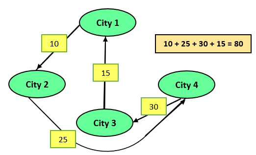
Let’s understand this with the help of an example. Given, City1, City2, City3, City4 and distances between them as shown below. A salesman has to start from City 1, travel through all the cities and return to City1. There are various possible paths, but the problem is to find the shortest possible route.
The various possible routes are:
Route
Distance Travelled
City(1 - 2 - 3 - 4 - 1)
95
City(1 - 2 - 4 - 3 - 1)
80
City(1 - 3 - 2 - 4 - 1)
95
Since we are travelling in a loop(source and destination are the same), paths like (1 - 2 - 3 - 4 - 1) and (1 - 4 - 3 - 2 - 1) are considered identical.
Out of the above three routes, route 2 is optimal. So, this will be the answer.
Let’s understand the solution approach to this problem.
Recommended: Try the Problem yourself before moving on to the solution
Solution Approach(Dynamic programming)
A dynamic programming paradigm is used when we have problems that can be decomposed into similar sub-problems. In this paradigm, the results of the subproblems are stored to reuse later. These algorithms are primarily used for optimization.
As we saw earlier, TSP is an optimization problem. To apply the DP technique, we need to find out if TSP can be divided into similar subproblems or not.
Let's take the above example. The graph and its cost adjacency matrix is given below:
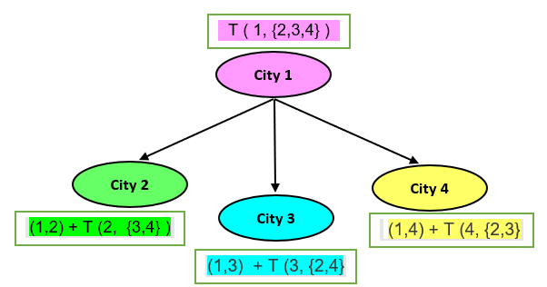
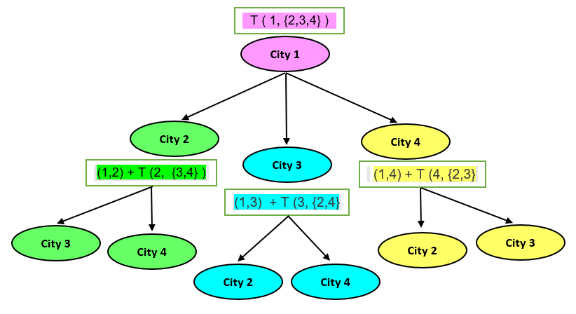
We can observe that the adjacency cost matrix is symmetric. By symmetric, we mean the distance between cities 2 to 3 is the same as cities 3 to 2. Let’s take a tour T from city 1 to any of the cities 2, 3, 4 as T (1,{2,3,4}). There are three possible ways to complete this tour.
Case 1: If he visits from City 1 to 2, this further depends on a subproblem, i.e. visiting from City 2 to City 3 or 4.
Case 2: If he visits from City 1 to 3, this further depends on a subproblem, i.e. visiting from City 3 to City 2 or 4.
Case 3: If he visits from City 1 to 4, this further depends on a subproblem, i.e. visiting from City 4 to City 2 or 3.
Here, we can observe that TSP can be divided into subproblems. This means we can use dynamic programming techniques to solve this problem.
Now, let’s see the dynamic programming approach in detail of the tour mentioned above:
Let the equation 1 be:
T ( 1, {2,3,4} ) = minimum of { (1,2) + T (2, {3,4} ), (1,3) + T (3, {2,4} ), (1,4) + T (4, {2,3} ) }
The above problem depends on some new subproblems. Let’s solve them first.
T (2, {3,4} ) = minimum of { (2,3) + T (3, {4} ), (2,4) + T {4, {3} ) }
(2,3) + T (3, {4} ) = 35 + 30 = 65 + 20(Cost of going back to 1) = 85
(2,4) + T {4, {3} ) = 25 + 30 = 55 + 15(Cost of going back to 1) = 70
T (2, {3,4} ) = minimum of { 85, 70 } = 70
T (3, {2,4} ) = minimum of { (3,2) + T (2, {4} ), (3,4) + T {4, {2} ) }
(3,2) + T (2, {4} ) = 35 + 25 = 60 + 20(Cost of going back to 1) = 80
(3,4) + T {4, {2} ) = 30 + 25 = 55 + 10(Cost of going back to 1) = 65
T (3, {2,4} ) = minimum of { 80, 65 } = 65
T (4, {2,3} ) = minimum of { (4,2) + T (2, {3} ), (4,3) + T {3, {2} ) }
(4,2) + T (2, {3} ) = 25 + 35 = 60 + 15(Cost of going back to 1) = 75
(4,3) + T {3, {2} ) = 30 + 35 = 65 + 10(Cost of going back to 1) = 75
T (4, {2,3} ) = minimum of { 75, 75 } = 75
Now putting the values of these subproblems in equation 1
T ( 1, {2,3,4} ) = minimum of { (1,2) + 70, (1,3) + 65,(1,4) + 75}
T ( 1, {2,3,4} ) = minimum of { 10 + 70, 15 + 65, 20 + 75}
T ( 1, {2,3,4} ) = minimum of {80, 80, 95} = 80
Here, the tour having the path 1 -> 2 -> 4 -> 3 -> 1 and 1 -> 3 -> 4 -> 2 -> 1 are same and having the minimum cost as 80.
Implementation
Here, we are using the DP array to store the results of the subproblems. We are using bit masking techniques to keep track of the cities that are visited.
#include<bits/stdc++.h>
using namespace std;

#define MAX 999999
//Number of Cities
int n=4;
//Adjacency Matrix of the graph
int Adj_matrix[10][10] = {
        {0,10,15,20},
        {10,0,35,25},
        {15,35,0,30},
        {20,25,30,0}
};
//Bit Mask to keep track of visited Cities
int Visited = (1<<n) - 1;
//DP Array to store the results of subproblem
int dp[16][4];

int  TSP_DP(int mask,int pos){
//If the city is already visited
    if(mask==Visited){
		return Adj_matrix[pos][0];
	}
//Lookup Case
	if(dp[mask][pos]!=-1){
	  return dp[mask][pos];
	}
//Now, from the current node, we will try to go to every
      //other node and take the min ans
	int ans = MAX;
	//Visit all the unvisited cities and take the best route
	for(int city=0;city<n;city++){
		if((mask&(1<<city))==0){
			int newAns = Adj_matrix[pos][city] + TSP_DP( mask|(1<<city), city);
			ans = min(ans, newAns);
			}
	}
	return dp[mask][pos] = ans;
}

int main(){

    //Initialisation of DP Array

    for(int i=0;i<(1<<n);i++)
    {
        for(int j=0;j<n;j++)
        {
            dp[i][j] = -1;
        }
    }
    //Starting city: 1, BitMask: 0
	cout<<"Minimum Cost is: "<<TSP_DP(1,0);
	return 0;
}
You can also try this code with Online C++ Compiler
The time complexityis O (n22n), where n is the number of cities.
Reason: While solving recursive equations, we will get a total (n-1) 2(n-2) sub-problems, which is O (n2n). Each sub-problem will take O (n) time to find a path to the remaining (n-1) cities.
Therefore total time complexity is O (n2n) * O (n) = O (n22n)
TSP is the travelling salesman problem consists of a salesperson and his travel to various cities. The salesperson must travel to each of the cities, beginning and ending in the same.
What type of problem is TSP?
TSP is an optimization problem. In this, we have to optimize the route of travel.
How is TSP related to the minimum spanning tree?
TSP and MST are two algorithmic problems that are closely connected. In particular, an open-loop TSP solution is a spanning tree, although it is not always the shortest spanning tree.
Conclusion
In this article, we ran you through the travelling salesman problem. We saw a dynamic programming approach to solve the problem.
There are various algorithmic paradigms such as Dynamic Programmingand Backtracking to solve this problem. We saw earlier that TSP is somewhat related to the minimum spanning tree. You can visit these two outstanding articles onPrims andKruskal's algorithm.


 9+ registered

