Understanding K-means through an Example
Let’s try understanding K-means through an example. In this example, we will be using some random datasets and the Scikit-learn library.
Step 1: Import the required libraries
import numpy as np
import matplotlib.pyplot as plt
%matplotlib inline

You can also try this code with Online Python Compiler
Here in the above code, we import the following libraries :
- NumPy: to perform efficient calculations on matrices.
-
matplotlib: to help visualize the data.
Step 2: Getting Random dataset
points= -2 * np.random.rand(100,2) # (will give values in range (-2, 0))
tmp1 = 1 + 2 * np.random.rand(50,2) # (will give values in range (1, 3))
points[50:100, :] = tmp1 #(making lower half values in range(1, 3))

# displaying the generated dataset
plt.scatter(points[ : , 0], points[ :, 1], s = 50, c = 'b')
plt.show()
You can also try this code with Online Python Compiler
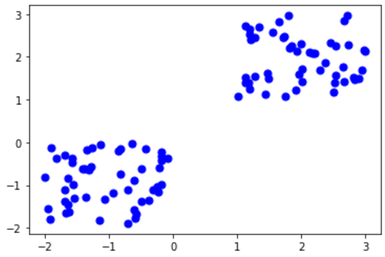
The above code generates random 100 data points divided into two different groups of 50 each. We have also displayed the generated data to help us visualize the clusters. Here is how the data points look in a 2D plane.
Step 3: Processing the Data and Computing K-means clustering
from sklearn.cluster import KMeans

Kmean = KMeans(n_clusters=2) # choosing k value arbitrarily clusters

# Compute k-means clustering.
Kmean.fit(points)
You can also try this code with Online Python Compiler
Here we use the available library function in scikit-learn to process the data.
Step 4: Finding the centroid of clusters
clusters_centers_ attribute of KMeans gives the center of the clusters.
# Coordinates of cluster centers.
Kmean.cluster_centers_
You can also try this code with Online Python Compiler
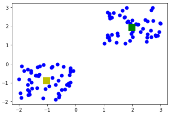
Here is the output for our data.
array([[-1.03169853, -0.88661647],
       [ 1.978359  ,  1.9484259 ]])
Let’s use matplotlib and visualize the centroids along with other data points on a 2D plane.
centroid0 = Kmean.cluster_centers_[0][:]
centroid1 = Kmean.cluster_centers_[1][:]
You can also try this code with Online Python Compiler
# Displaying the cluster centroids (using yellow and blue color)
plt.scatter(points[ : , 0], points[ : , 1], s=50, c='b')
plt.scatter(centroid0[0], centroid0[1], s=200, c='y', marker='s')
plt.scatter(centroid1[0], centroid1[1], s=200, c='g', marker='s')
plt.show()
You can also try this code with Online Python Compiler
Output
Step 5: Testing the algorithm
Let’s display the label of each data point that was in our dataset.
# Labels of each point
Kmean.labels_
You can also try this code with Online Python Compiler
Output
array([0, 0, 0, 0, 0, 0, 0, 0, 0, 0, 0, 0, 0, 0, 0, 0, 0, 0, 0, 0, 0, 0,
       0, 0, 0, 0, 0, 0, 0, 0, 0, 0, 0, 0, 0, 0, 0, 0, 0, 0, 0, 0, 0, 0,
       0, 0, 0, 0, 0, 0, 1, 1, 1, 1, 1, 1, 1, 1, 1, 1, 1, 1, 1, 1, 1, 1,
       1, 1, 1, 1, 1, 1, 1, 1, 1, 1, 1, 1, 1, 1, 1, 1, 1, 1, 1, 1, 1, 1,
       1, 1, 1, 1, 1, 1, 1, 1, 1, 1, 1, 1])
From the output, we can infer that the first 50 points are in cluster 0 and the next 50 in cluster 1. This can also be verified from the figure in which we displayed data points on a 2D plane.
Now let us take a random point and predict the cluster to which its more closer.
data_point=np.array([-2.0,-2.0])
test_points=data_point.reshape(1, -1)

# Predict the closest cluster each sample in sample_test belongs to
Kmean.predict(test_points)
You can also try this code with Online Python Compiler
Output
array([0])
Output shows that (-2, -2) belongs to cluster 0 (i.e nearer to yellow centroid)
You can find the complete code here.
Disadvantages in Using K-Means
For data cluster analysis, K-means clustering is a widely used technique.
However, slight alterations in the data might lead to considerable variance, so its performance is usually not as good as that of other complex clustering algorithms.
Furthermore, clusters are considered spherical and uniform in size, which could lower the precision of the K-means clustering Python findings.
Key Takeaways
Cheers if you reached here!! In this blog, we used a random dataset to understand how the K-Means clustering algorithm works.
Yet learning never stops, and there is a lot more to learn. Happy Learning!!


 8+ registered

