Uniform and Exponential Distribution

Random Variable

A random variable's possible values are numerical results of an unexpected event. Discrete and Continuous random variables are the two forms of random variables.

A discrete random variable can only have a finite number of different values and can thus be quantified. For example, a random variable X can be defined as the number that appears when a fair dice is rolled. X can only take values: 1,2,3,4,5, or 6.

To make a mathematical sense, suppose a random variable X may take k number of different values, with the probability that X=x_i is defined to be P(X==x_i)=p_i. Then the probabilities p_i must satisfy the following:

• Each p_i  should be in the range 0 < pi < 1.
• Σp_i =1

A continuous random variable can take an endless number of different values. For example, a random variable X can be defined as pupils' height in a class. The area under a curve represents a continuous random variable because it is illustrated throughout a range of values (or the integral).

Probability distribution functions take on continuous values and represent the probability distribution of a continuous random variable. Because the number of possible values for the random variable is unlimited, the probability of seeing any single value is zero. A random variable X, for example, could take any matter within a range of natural integers.
 

The curve that represents the function p(x) must meet the following requirements:

• p(x)>0 for all x 
• The entire area beneath the curve is one.

source

Uniform Distribution

The uniform distribution is a probability distribution in which all values within a specific range are equally likely to occur, whereas values outside the scope are never seen. When we plot the density of a uniform distribution, we know that it is flat since no value is more likely (and so has more density) than the others.

Ex:

Flying time from Newark to Atlanta runs from 120 to 150 minutes, with a very regular distribution if we track the flight time for many commercial flights.

Source

Using scipy, you may construct a uniform distribution in Python by first importing the necessary libraries.

%matplotlib inline

 
import numpy as np
import pandas as pd
import matplotlib.pyplot as plt
import scipy.stats as stats

 
uniform_data_dist = stats.uniform.rvs(size=10000,  # Generate 10000 numbers
                                 loc = 0,      # From 0 
                                 scale=10)     # To 10
 # Plot the distribution
pd.DataFrame(uniform_data_dist).plot(kind="density", 
                               figsize=(9,9),
                               xlim=(-5,15));

You can also try this code with Online Python Compiler

Run Code

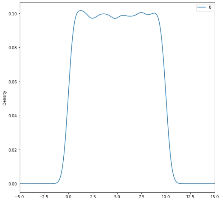
Because it is based on a sample of observations, the graphic above represents an approximation of the underlying distribution.

We created data points from a uniform distribution in a specific range using the code above. The density of our uniform data is virtually flat on the density plot, indicating that any given value has the same likelihood of happening.

Normal Distribution

Continuous probability distribution with a symmetric bell-shaped curve is known as the normal or Gaussian distribution. The center (mean) and spread of a normal distribution describe it (standard deviation.). The majority of the observations generated by a normal distribution are close to the mean, which is located in the exact center of the distribution:

On average, about 68 percent of the data is within one standard deviation of the mean.

95 percent is within two standard deviations.

99.7% is within three standard deviations.

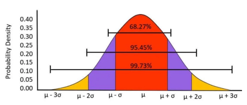
Normal distribution

In all of statistics, the normal distribution is possibly the most important distribution. Many real-world events, such as IQ test scores and human heights, follow a normal distribution, which is why it is frequently employed to describe random variables.

Ex : Examples: Performance appraisal, Height, BP, measurement error , and IQ scores follow a normal distribution.

The normal distribution mathematical formula is as follows: (read: miu) is the mean, and (read: sigma) is the deviation of the data.

Formula

By first loading the appropriate libraries, you may generate a normal distribution in Python using scipy:

from scipy.stats import norm
import seaborn as sns
import matplotlib.pyplot as plt

 
normal_dist = norm.rvs(size=100000,loc=0,scale=1)

 
sns.distplot(normal_dist,
              kde=True,
              bins=100,
              color='red',
              hist_kws={"linewidth": 15,'alpha':1});

You can also try this code with Online Python Compiler

Run Code

The bell shape of the normal distribution is depicted in the graph above

FAQs

1. What Is a Uniform Distribution's Expectation?
   A uniform distribution is anticipated to result in all conceivable outcomes having the same probability. One variable's probability is the same as another's.
    
2. What's the distinction between a normal and a uniform distribution?
   The most likely value is at the center of a normal distribution, which has a bell shape. A uniform distribution is flat, with all values having the same probability.
    
3. What exactly does the word distribution signify?
   Distribution shows how values disperse in series and how frequently they appear in this series.
    
4. What is the uniform distribution mode?
   Consider the case of an observation with a uniform distribution. The uniform distribution's probability density function, on the other hand, is constant. That is, (1/b-a). Therefore mode is not meaningful in this context.

Key Takeaways

The scipy library in Python offers functions that make working with a variety of probability distributions simple, including those that we didn't cover in this course. Probability distribution functions can be used to generate random data, simulate random events, and facilitate statistical testing and analysis.

You can learn more about them here.