Do you think IIT Guwahati certified course can help you in your career?
Introduction
Visual Geometry Group (VGG) was created to improve the model's performance by increasing the depth of such CNNs.
Deep learning has demonstrated great success in a wide range of computer vision applications in recent years. The discipline of machine learning has risen in prominence since then. The superior performance of deep learning algorithms over traditional machine learning algorithms opens up new possibilities in image recognition, CV, speech or voice recognition, translations, imaging in the medical field, robotics, and various other domains.
VGG stands for Visual Geometry Group, and it is part of Oxford University's Department of Science and Engineering. From VGG16 to VGG19, it has produced a series of convolutional network models that can be used for face recognition and picture categorization. The VGG architecture serves as the foundation for cutting-edge object recognition models. The VGGNet, which was created as a deep neural network, outperforms baselines on a variety of tasks and datasets in addition to ImageNet. Furthermore, it is still one of the most widely used image recognition architectures today.
The VGG model, often known as VGGNet, is a convolutional neural network model proposed by A. Zisserman and K. Simonyan of the University of Oxford that supports 16 layers. The model was reported in the publication "Very Deep Convolutional Networks for Large-Scale Image Recognition" by these researchers. In ImageNet, the VGG16 model achieves about 92.7 percent top-5 test accuracy. ImageNet is a collection with about 14 million photos divided into over 1000 categories. It was also one of the most popular models submitted to the 2014 ILSVRC. It makes considerable improvements over AlexNet by replacing big kernel-sized filters with numerous 33 kernel-sized filters one after the other. The VGG16 model was trained over several weeks using Nvidia Titan Black GPUs.
The VGG19 model (also known as VGGNet-19) is similar to the VGG16, but it has 19 layers. The numbers "16" and "19" refer to the model's weight layers (convolutional layers). VGG19 contains three additional convolutional layers than VGG16. In the second half of this post, we'll go through the properties of VGG16 and VGG19 networks in greater depth.
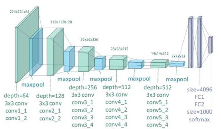
A 224*224 RGB image is used as the input to the VGG-based convNet. Preprocessing layer takes the RGB image with pixel values in the range of 0–255 and subtracts the mean image values which is calculated over the entire ImageNet training set.
After preprocessing, the input photos are transmitted via these weight layers. A stack of convolution layers is used to send the training images through. In the VGG16 architecture, there are a total of 13 convolutional layers and three fully connected layers. Instead of having huge filters, VGG features smaller filters (3*3) with better depth. It now has the same effective receptive field as if only one 7 × 7 convolutional layers were used.
A tour of the architecture in a more detailed manner:
The VGGNet accepts an image input size of 224x224 pixels. To keep the image input size consistent for the ImageNet competition, the model's authors chopped out the middle 224x224 patch in each image.
Convolutional Layers: VGG's convolutional layers use a small receptive field (33), the smallest size that still captures up/down and left/right movement. In addition, there are 11 convolution filters that operate as a linear transformation of the input. Then there's a ReLU unit, which is a significant AlexNet invention that cuts training time in half. The rectified linear unit activation function (ReLU) is a piecewise linear function that outputs the input if it is positive and zero otherwise. To maintain spatial resolution after convolution, the convolution stride is set to 1 pixel (stride is the number of pixel shifts over the input matrix).
The VGG network's hidden layers all use ReLU. Local Response Normalization (LRN) is rarely used in VGG preprocessing since it increases memory usage and training time. Furthermore, it has no effect on total accuracy.
The VGGNet is made up of three layers that are all fully connected. The first two layers each have 4096 channels, whereas the third layer contains 1000 channels, one for each class.
VGG brings with it a variety of structures based on the same idea. This provides us additional alternatives when it comes to determining which architecture would work best for our application.
Non-linearity increased as the number of layers with smaller kernels increased, which is always a good thing in deep learning.
VGG resulted in a significant increase in accuracy as well as a significant increase in speed. This was mostly due to the model's increased depth and the addition of pretrained models.
Disadvantages of VGG
This model suffers from the vanishing gradient problem, which I discovered to be a significant drawback. When we look at my validation loss graph, we can see that it is steadily growing. None of the other models were in the same boat. The ResNet architecture was used to tackle the vanishing gradient problem.
The older VGG design is slower than the newer ResNet architecture, which introduced the idea of residual learning, another key accomplishment.
Implementation
# importing all libraries required

from tensorflow.keras.layers import Input, Conv2D, MaxPooling2D
from tensorflow.keras.layers import Dense, Flatten
from tensorflow.keras.models import Model

_input = Input((224,224,1))  #INPUT IMAGE SHAPE
You can also try this code with Online Python Compiler
# Working with a model that has already been trained(pretrained)
from keras.applications.vgg16 import decode_predictions
from keras.applications.vgg16 import preprocess_input
from keras.preprocessing import image
import matplotlib.pyplot as plt
from PIL import Image
import seaborn as sns
import pandas as pd
import numpy as np
import os

img1 = "../input/flowers-recognition/flowers/tulip/10094729603_eeca3f2cb6.jpg"
img2 = "../input/flowers-recognition/flowers/dandelion/10477378514_9ffbcec4cf_m.jpg"
img3 = "../input/flowers-recognition/flowers/sunflower/10386540696_0a95ee53a8_n.jpg"
img4 = "../input/flowers-recognition/flowers/rose/10090824183_d02c613f10_m.jpg"
imgs = [img1, img2, img3, img4]

def _load_image(img_path):
    img = image.load_img(img_path, target_size=(224, 224))
    img = image.img_to_array(img)
    img = np.expand_dims(img, axis=0)
    img = preprocess_input(img)
    return img

def _get_predictions(_model):
    f, ax = plt.subplots(1, 4)
    f.set_size_inches(80, 40)
    for i in range(4):
        ax[i].imshow(Image.open(imgs[i]).resize((200, 200), Image.ANTIALIAS))
    plt.show()

    f, axes = plt.subplots(1, 4)
    f.set_size_inches(80, 20)
    for i,img_path in enumerate(imgs):
        img = _load_image(img_path)
        preds  = decode_predictions(_model.predict(img), top=3)[0]
        b = sns.barplot(y=[c[1] for c in preds], x=[c[2] for c in preds], color="gray", ax=axes[i])
        b.tick_params(labelsize=55)
        f.tight_layout()

from keras.applications.vgg16 import VGG16
vgg16_weights = '../input/vgg16/vgg16_weights_tf_dim_ordering_tf_kernels.h5'
vgg16_model = VGG16(weights=vgg16_weights)
_get_predictions(vgg16_model)
You can also try this code with Online Python Compiler
Please note that Alexnet is quite unlikely to outperform VGG. One option is that VGG's hyper-parameter tweaking isn't done properly, whereas Alexnet's tuning is superior.
Why can't three 3x3 convolutions take the place of seven 7x7 convolutions?
3x3 convolutions with 3 non-linear activation functions, boosting non-linear expression possibilities and separability of the segmentation plane Reducing the number of parameters is a good idea. 7x7 provides parameters for the convolution kernel of C channels, and the number of 3x3 parameters is considerably decreased.
What is the role of a 1x1 convolution kernel?
Increase the model's nonlinearity while keeping the receptive field same. The non-linear activation function plays a non-linear role in a 1x1 winding machine, which is comparable to linear transformation.
What is Local Response Normalization?
Local Response Normalization (LRN) was originally employed in AlexNet architecture, where ReLU was used as the activation function rather than the more usual tanh and sigmoid at the time. Apart from the reasons stated above, the use of LRN was intended to promote lateral inhibition.
What is the difference between BN(Batch Normalization) and LRN(local response normalization)?
LRN, on the other hand, has numerous ways to achieve normalization (Inter or Intra Channel), but BN only has one (for each pixel position across all the activations).
Conclusion
This blog covered VGG extensively which is a cutting-edge object-recognition model with up to 19 layers. VGG, which was built as a deep CNN, outperforms baselines on a variety of tasks and datasets outside of ImageNet. VGG is one of the most widely used image-recognition models today. To know more about such concepts check out our machine learning blogs. Do upvote our blog to help other ninjas grow. Happy coding!


 9+ registered

