Do you think IIT Guwahati certified course can help you in your career?
Introduction
Deep learning neural networks tend to be opaque; thus, even if they can make accurate predictions, it is often unclear how or why a particular prediction was formed. Convolutional neural networks keep the spatial relationships for what the model learns because its internal structures are made to operate on two-dimensional picture data. In particular, the model's two-dimensional filters may be examined and visualized to determine the features it will detect, and convolutional layer activation maps can be reviewed to see precisely which features were recognized for a specific input image.
In this article, you will learn how to create straightforward visualizations for filters and feature maps in a convolutional neural network.
Whether it's a tree-based model or a sizable neural network, visualizing the output of your machine learning model is a terrific method to understand how it's progressing. Most people only consider the training error (accuracy) and validation error while training deep networks (accuracy). There is so much more that we can view and thus learn about network architecture when it comes to deep CNN networks like Inception. Judging these two aspects does offer us a sense of how our network is functioning at each epoch.
Visualizing Intermediate Layer Activations
We need to understand how our deep convolutional neural network model perceives the input image by examining the output of its intermediate layers to comprehend how our model can classify the input image. By doing this, we can discover more about how these layers function.
Some filters function as edge detectors, while others focus on a specific area of the flower, such as the center, and yet others serve as background detectors. Since the pattern caught by the convolution kernel becomes sparser as you go deeper, it is simpler to observe this behavior of convolution layers in the initial layers. However, it is possible that such patterns may not even exist in your image, in which case they would not be collected.
Visualizing Convnet Filters
Visualizing the convolution layer filters is another approach to understanding what your convolution network is looking for in the photos. By presenting the network layer filters, you may discover the pattern that each filter will respond to. Starting with a blank input image, this can be accomplished by applying Gradient Descent on the value of a convnet to maximize the response of a particular filter.
Visualizing Heatmaps of class activations
When predicting the class labels for photos, your model may occasionally predict the incorrect label for your class, meaning the probability of the correct label is not always at its highest. When this happens, it will be beneficial if you can see what parts of the image your convnet is analyzing to get the class labels.
Class Activation Map (CAM) visualization is the umbrella term for this class of methods. Making heatmaps of class activations across input photos is one of the CAM approaches. A class activation heatmap is a 2D grid of scores computed for each place in an input image and assigned to a specific output class that shows how significant each location is concerning that output class.
Visualizing Convolutional Layers
Opaque is a standard description of neural network models. This indicates that they do poorly elaborates on the rationale behind a given judgment or prediction. Convolutional neural networks are intended to process picture input, and given that, they should be easier to understand than other varieties of neural networks. The models are made up of tiny linear filters and the output of applying filters known as activation maps, or more generally, feature maps. Visualizing filters and feature maps is possible. For example, we can create and comprehend tiny filters like line detectors. A learned convolutional neural network's filters may be visualized to help explain the model's operation.
The feature maps produced by applying filters to input images and feature maps produced by earlier layers may shed light on the internal representation of a particular input that the model possesses at a certain stage. In this article, we will examine both of these methods for convolutional neural network visualization.
Pre-fit VGG Model
For visualization, we require a model. We can employ a pre-fit previous state-of-the-art image classification model rather than creating a model from the start.
For the ILSVRC (stands for ImageNet Large Scale Visual Recognition Challenge), several examples of effective picture classification models created by various research teams are provided by Keras. The VGG-16 model, which won the 2014 competition, is one example. Because it has a straightforward uniform structure of sequentially ordered convolutional and pooling layers, is deep (16 learned layers), and performs well, this model is a strong choice for visualization because it will capture valuable information in the filters and feature maps that result.
# load vgg model
from keras.applications.vgg16 import VGG16
# load the model
model = VGG16()
# summarize the model
model.summary()
When we run the example, the model weights are loaded into memory, and a summary of the loaded model is printed. The weights will be obtained from the internet and saved in your home directory if this is your first time loading the model. These files weigh about 500 megabytes and, depending on your internet connection speed, can take a while to download.
The layers' names are clear, they are arranged into blocks, and names for each block's layers use integer indices. We can utilize the pre-fit model we have created as the foundation for visualizations at this point.
How to Visualize Filters
Plotting the learned filters is maybe the most straightforward visualization to complete. The learned filters are only weights in the context of neural networks. Still, because of their unique two-dimensional structure, the weight values have a spatial relationship, making it worthwhile to display each filter as a two-dimensional image (or could be). The first step is reviewing the model's filters to determine what we have to work with.
The output shape of each layer, such as the shape of the generating feature maps, is summarized in the model summary written in the preceding section. Only the total number of weights per layer is shown, with no indication of the form of the filters (weights) in the network. The model provides access to all of the model's layers characteristics of layers.
Convolutional layers have naming conventions like block# conv#, where the '#' is an integer, and each layer has a layer.name property. As a result, we may examine each layer's name and disregard any that do not contain the word "conv."
# summarize filter shapes
for layer in model.layers:
    # check for convolutional layer
    if 'conv' not in layer.name:
        continue
The weights in each convolutional layer come in two groups. The block of filters is one, and the block of bias values is another. Through the layer.get weights() function, you can access these. These weights are retrievable, and we can summarize their shape after that.
# get filter weights
filters, biases = layer.get_weights()
print(layer.name, filters.shape)
Summarizing the model filters complete example is provided below.
# summarize filters in each convolutional layer
from keras.applications.vgg16 import VGG16
from matplotlib import pyplot
# load the model
model = VGG16()
# summarize filter shapes
for layer in model.layers:
    # check for convolutional layer
    if 'conv' not in layer.name:
        continue
    # get filter weights
    filters, biases = layer.get_weights()
    print(layer.name, filters.shape)
When the example is run, a list of layer specifics is printed, including the layer name and the form of the layer's filters.
We can see that 33 filters, which are compact and potentially simple to understand, are used by all convolutional layers. A convolutional neural network's architectural issue is that a filter's depth must coincide with the filter's input depth (e.g., the number of channels). We can see that each filter has a depth of three for the input image, with three channels for red, green, and blue (here, we are working with a channel-last format). The first layer's filters are retrievable as follows:
# retrieve weights from the second hidden layer
filters, biases = model.layers[1].get_weights()
The weight values will probably have modest positive and negative values near 0.0. To make them simpler to visualize, we can normalize their values to the range 0–1.
# normalize filter values to 0-1 so we can visualize them
f_min, f_max = filters.min(), filters.max()
filters = (filters - f_min) / (f_max - f_min)
The first six filters out of the total 64 in the block may now be listed, and each filter's three channels can be plotted. Each filter is plotted using the matplotlib library as a new row of subplots and a new column for each filter channel or depth.
# plot first few filters
n_filters, ix = 6, 1
for i in range(n_filters):
    # get the filter
    f = filters[:, :, :, i]
    # plot each channel separately
    for j in range(3):
        # specify subplot and turn of axis
        ax = pyplot.subplot(n_filters, 3, ix)
        ax.set_xticks([])
        ax.set_yticks([])
        # plot filter channel in grayscale
        pyplot.imshow(f[:, :, j], cmap='gray')
        ix += 1
# show the figure
pyplot.show()
You can also try this code with Online Python Compiler
The VGG16 model's full example of charting the first six filters from the hidden convolutional layer is shown below.
# cannot easily visualize filters lower down
from keras.applications.vgg16 import VGG16
from matplotlib import pyplot
model = VGG16()
filters, biases = model.layers[1].get_weights()

f_min, f_max = filters.min(), filters.max()
filters = (filters - f_min) / (f_max - f_min)
n_filters, ix = 6, 1
for i in range(n_filters):
    # get the filter
    f = filters[:, :, :, i]
    # plot each channel separately
    for j in range(3):
        # specify subplot and turn of axis
        ax = pyplot.subplot(n_filters, 3, ix)
        ax.set_xticks([])
        ax.set_yticks([])
        # plot filter channel in grayscale
        pyplot.imshow(f[:, :, j], cmap='gray')
        ix += 1
# show the figure
pyplot.show()
You can also try this code with Online Python Compiler
When the example is run, a figure is produced that contains six rows of three images, one column for each channel and one row for each filter. In some instances, we can see that (the first row), the filter is the same across all of the channels, whereas, in other cases, the filters vary (the last row). Small or inhibitory weights are shown by dark squares, whereas light squares show big or excitatory weights. This understanding allows us to observe that the first row's filters pick up on a gradient from light in the top left to dark in the bottom right. Source
Despite having a visualization, we can only make out the first six of the first convolutional layer's 64 filters. It is possible to see all 64 filters in a single photograph. Unfortunately, this does not scale. If we want to start looking at filters in the second convolutional layer, we can see that there are once again 64 filters, but each has 64 channels to match the input feature maps. It may be difficult to discern any detail in (6464) 4,096 subplots needed to view all 64 channels in a row for all 64 filters.
How to Visualize Feature Maps
The activation maps, also known as feature maps, record what happens when the filters are applied to an input, either the input image or another feature map. Understanding what input features are recognized or preserved in the feature maps is the goal of seeing a feature map for a particular input image. In contrast to feature maps close to the model's output, which would be expected to capture more generic features, feature maps close to the input would likely identify small or fine-grained detail.
We require input for the VGG16 model that may be used to generate activations so that we can investigate the visualization of feature maps. We'll make use of a clear image of a bird.
Bird Image(Robin by Chris Heald)
Next, to extract the correct layer output, we need a better understanding of the shape of the feature maps produced by each convolutional layer and the layer index number. The sample below will list every layer in the model, print the size of each convolutional layer's output or feature map, and display the layer index.
# summarize feature map size for each conv layer
from matplotlib import pyplot
from keras.applications.vgg16 import VGG16

model = VGG16()

for i in range(len(model.layers)):
    layer = model.layers[i]
    # check for convolutional layer
    if 'conv' not in layer.name:
        continue
    # summarize output shape
    print(i, layer.name, layer.output.shape)
You can also try this code with Online Python Compiler
Using this knowledge, we can create a new model that has only a portion of the layers included in the entire VGG16 model. The output of a particular convolutional layer, which we know would be the activation of the layer or the feature map, would be different from the model's input layer, which would remain the same as in the original model.
A new model that generates a feature map from the first convolutional layer (index 1), for instance, can be defined as follows after loading the VGG model.
# redefine model to output
model = Model(inputs=model.inputs, outputs=model.layers[1].output)
You can also try this code with Online Python Compiler
The feature map for the first convolutional layer for a particular input image will be provided when making a prediction using this model. Implementing this now.
After defining the model, we must load the bird image at the 224X224 resolution that the model requires.
The image PIL object must then be expanded from a 3D array to a 4D array with the dimensions [samples, rows, cols, channels], where we only have one sample, then transformed to a NumPy array of pixel data.
# convert the image to an array
img = img_to_array(img)
# expand dimensions
img = expand_dims(img, axis=0)
You can also try this code with Online Python Compiler
After that, the pixel values must be scaled properly for the VGG model. Now is the time to obtain the feature map. Calling the model makes it simple for us to do this. Using the predict() function with the provided single image as input.
# prepare the image
img = preprocess_input(img)
# get a feature map for the first hidden layer
feature_maps = model.predict(img)
You can also try this code with Online Python Compiler
We are aware that the outcome will be a 224x224x64 feature map. All 64 two-dimensional images can be plotted as an 8 by 8 square.
# plot all 64 maps in 8x8
square = 8
ix = 1
for _ in range(square):
    for _ in range(square):
        ax = pyplot.subplot(square, square, ix)
        ax.set_xticks([])
        ax.set_yticks([])
        pyplot.imshow(feature_maps[0, :, :, ix-1], cmap='gray')
        ix += 1
pyplot.show()
You can also try this code with Online Python Compiler
The entire code example for viewing the feature map for the first convolutional layer in the VGG16 model for an input image of a bird is provided below.
# plot feature map of
#first conv layer for a given image
from keras.applications.vgg16 import preprocess_input
from keras.applications.vgg16 import VGG16
from keras.preprocessing.image import img_to_array
from keras.preprocessing.image import load_img
from matplotlib import pyplot
from keras.models import Model
from
numpy import expand_dims
model = VGG16()

model = Model(inputs=model.inputs, outputs=model.layers[1].output)
model.summary()
img = load_img('bird.jpg', target_size=(224, 224))

img = img_to_array(img)
# expand dimensions
img = expand_dims(img, axis=0)
# prepare the image
img = preprocess_input(img)
# get a feature map for the first hidden layer
feature_maps = model.predict(img)
# plot all 64 maps in 8x8
square = 8
ix = 1
for _ in range(square):
    for _ in range(square):
        # specify subplot and turn of axis
        ax = pyplot.subplot(square, square, ix)
        ax.set_xticks([])
        ax.set_yticks([])
        pyplot.imshow(feature_maps[0, :, :, ix-1], cmap='gray')
        ix += 1
pyplot.show()
You can also try this code with Online Python Compiler
Running the example first provides an overview of the new, more compact model that processes an image to produce a feature map. Remember that while being considerably smaller than the VGG16 model, this one employs the same weights (filters) in the first convolutional layer. The 64 feature maps are then represented as subplots in a figure. We can observe that a variety of variations of the bird image with various features highlighted are produced as a result of applying the filters in the first convolutional layer. Source
This is an intriguing outcome that mostly meets our expectations. The example could be updated to plot the feature maps produced by the output of further particular convolutional layers. Another strategy would be to make images of all the feature maps that were output from each block of the model in a single run. The image has a pooling layer at the end of five main blocks (block1, block2, etc.). The last convolutional layer in each block has the layer indices [2, 5, 9, 13, 17].
A list of feature maps will be produced after making a prediction using this new model. We are aware that deeper layers include considerably more feature maps than 64, like 256 or 512, such as depth or the number of channels. However, for consistency, we can limit the number of feature maps displayed to 64.
# plot the output from each block
square = 8
for fmap in feature_maps:
    # plot all 64 maps in 8x8 squares
    ix = 1
    for _ in range(square):
        for _ in range(square):
            # specify subplot and turn of axis
            ax = pyplot.subplot(square, square, ix)
            ax.set_xticks([])
            ax.set_yticks([])
            # plot filter channel in grayscale
            pyplot.imshow(fmap[0, :, :, ix-1], cmap='gray')
            ix += 1
    # show the figure
    pyplot.show()
You can also try this code with Online Python Compiler
By combining these modifications, we are now able to produce five distinct plots—one for each of the five blocks in the VGG16 model—for our bird shot. Below is a list of everything in it.
# visualize feature maps output
# from each block in the vgg model
from keras.applications.vgg16 import VGG16
from keras.preprocessing.image import load_img
from keras.applications.vgg16 import preprocess_input
from keras.models import Model
from keras.preprocessing.image import img_to_array
from matplotlib import
pyplot
from keras.models import Model
from numpy import expand_dims
model = VGG16()
# redefine model to output
ixs = [2, 5, 9, 13, 17]
outputs = [model.layers[i].output for i in ixs]
model = Model(inputs=model.inputs, outputs=outputs)
img = load_img('bird.jpg', target_size=(224, 224))
img = img_to_array(img)
# expand dimensions
img = expand_dims(img, axis=0)
# prepare the image
img = preprocess_input(img)
# get a feature map for the first hidden layer
feature_maps = model.predict(img)
# plot the output from each block
square = 8
for fmap in feature_maps:
    # plot all 64 maps in 8x8 squares
    ix = 1
    for _ in range(square):
        for _ in range(square):
            # specify subplot and turn of axis
            ax = pyplot.subplot(square, square, ix)
            ax.set_xticks([])
            ax.set_yticks([])
            # plot filter channel in grayscale
            pyplot.imshow(fmap[0, :, :, ix-1], cmap='gray')
            ix += 1
    # show the figure
    pyplot.show()
You can also try this code with Online Python Compiler
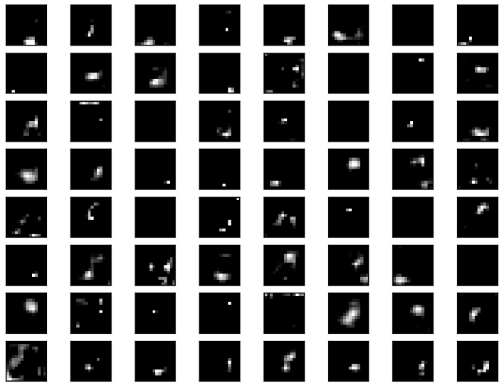
Five plots displaying the feature maps from the VGG16 model's five main blocks are produced after running the example. We can observe that as we move deeper into the model, the feature maps display less and less detail, whereas those closer to the model's input capture a lot of fine detail in the image. As the model abstracts the features from the image into broader ideas that may be utilized to generate a classification, this pattern was to be expected. We typically lose the ability to decipher these deeper feature maps, even when it is not immediately apparent from the final image that the model spotted a bird. Source
Block 1 - Visualization of the Feature Maps Extracted
Block 2 - Visualization of the Feature Maps Extracted
Block 3 - Visualization of the Feature Maps Extracted
Block 4 - Visualization of the Feature Maps Extracted
Block 5 - Visualization of the Feature Maps Extracted
Frequently Asked Questions
What do convolutional neural networks' filters do?
The function of a filter is to serve as a single template or pattern that, when convolved across the input, identifies correspondences between the stored template and various locations/regions in the input image.
How do convolutional neural networks learn the filters?
This is achieved by being familiar with the various levels of visual abstraction. The CNN often recognizes broad patterns in the first few hidden layers, such as edges; as we go deeper into the CNN, these learned abstractions get more precise, such as textures, patterns, and (parts of) things.
How many filters does a convolutional neural network have?
Filters help us better grasp what CNN is seeking to discover. AlexNet's initial convolution layer discovered these 96 filters.
Why do we employ several filters in convolutional neural networks?
It is more convenient to employ all necessary filters at once because convolving individual filters separately will lengthen calculation time.
Conclusion
In this article, we have extensively discussed the convolutional neural network. We have also explained how to enter visualizations in CNN, visualize convolutional layers, pre-fit the VGG model, visualize filters, and more in detail.


 8+ registered

