


Introduction
Before going on to the topic, let us revise what perceptron is. Perceptron is the simple model in an artificial neural network(ANN). In other words, it is an algorithm in supervised learning that helps in binary classification and multi-class classification.
There are two types of perceptrons. They are as follows:
- Single-layered perceptron.
- Multi-layered perceptron.
Let us see about these two models in detail.
Single-layered perceptron
A single-layered perceptron is a simple artificial neural network that includes only a forward feed. This model works on the threshold transfer function. It is one of the easiest artificial neural networks used in the binary classification of linearly separable objects. The output of the model is 1 or 0.
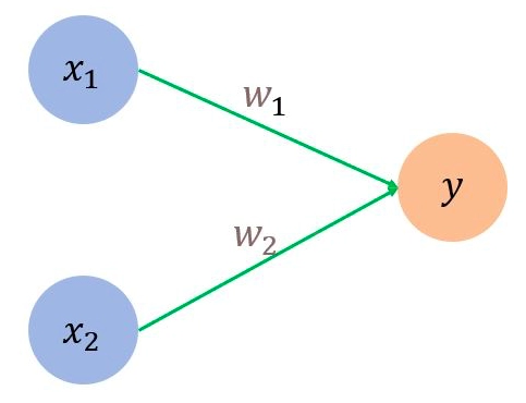
The single-layered perceptron doesn't have any previous information. It includes only two layers one is input, and another is output. The output is determined by the sum of the product of weights and input values. Below is the simple structure of a single-layered perceptron. (w1 & w2 are initialized randomly)
source
In the above figure, x1 and x2 are inputs of the perceptron, and y is the result. w1 and w2 are weights of the edges x1-y and x2-y. Let us define a threshold limit 𝛳. If the value of y exceeds the threshold value, the output will be 1. Else the output will be 0.
The equation is as follows.
y = x1*w1 + x2*w2
If y > 𝛳: output is 1
y ≤ 𝛳: output is 0.
Furthermore, weights are updated to minimize the error using the perceptron learning rule. The rule states that the algorithm automatically updates the optimal weight coefficient.
Let us understand the single-layered perceptron network by implementing the AND function.
Implementing AND function
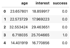
Let x1 and x2 be the input of the AND function. The values of x1 and x2 are shown below.
| x1 | x2 | y |
| 1 | 1 | 1 |
| 1 | 0 | 0 |
| 0 | 1 | 0 |
| 0 | 0 | 0 |
Let us import essential libraries for preparing the model.
|
import numpy as np # for plotting the graphs # for implementing perceptron model |
Preparing the dataset.
|
x1 = [1, 0, 0, 1] x2 = [1, 0, 1, 0] |
Perceptron model do not accept the above format of the data. Let us convert it into the proper format.
|
x = [[1,1], [0,0], [0, 1], [1, 0]] y = [1, 0, 0, 0] |
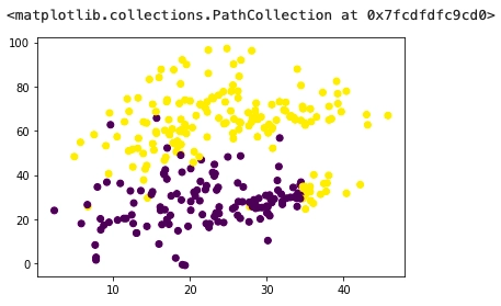
Checking whether the AND function is linearly separable.
|
plt.figure(figsize=(3, 3), dpi=80) plt.xlabel("x1") plt.ylabel("x2") plt.scatter(x1, x2, c = y) |
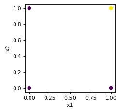
The above plot clearly shows that the AND function is linearly separable.
Let us draw a decision boundary to easily distinguish between the output(1 and 0).
Training the data.
| clf = Perceptron(max_iter=100).fit(x, y) |
After training the dataset we will print the information of the model.
|
print("Classes of the model : ",clf.classes_) print("Intercept of the decision boundary : ",clf.intercept_) print("Coefficients of the decision boundary : ",clf.coef_) |
|
Classes of the model : [0 1] Intercept of the decision boundary : [-2.] Coefficients of the decision boundary : [[2. 1.]] |
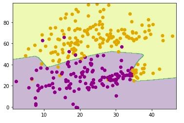
Plotting the decision boundary
|
# line segment ymin, ymax = -1,2 w = clf.coef_[0] a = -w[0] / w[1] xx = np.linspace(ymin, ymax) yy = a * xx - (clf.intercept_[0]) / w[1] # plotting the decision boundary plt.figure(figsize=(4, 4)) ax = plt.axes() ax.scatter(x1, x2, c = y) plt.plot(xx, yy, 'k-') ax.set_xlabel('X1') ax.set_ylabel('X2') plt.show() |
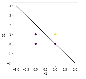
We can see the decision boundary classifies the four points. If x1 & x2 are 1, the output will be 1, and in the rest of the cases, the output is 0. Therefore, the yellow point with output 1 is separated from the purple data points with 0 output.


 8+ registered

