Using VLOOKUP in Excel
The purpose is to look up the table vertical. It searches based on the first index of the table and retrieves the column_index supplied in the arguments.
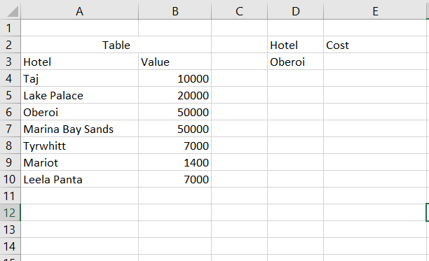
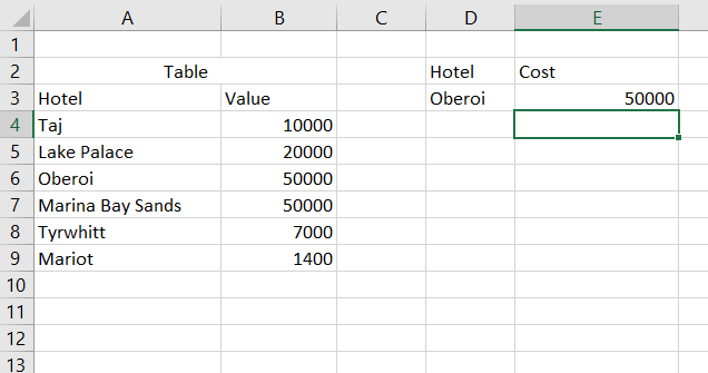
Consider the given table consisting of Hotel and Price.

We want to find the cost of Hotel Oberoi.
The syntax for VLOOKUP is =VLOOKUP(lookup_value,table,column_index, [range_lookup])
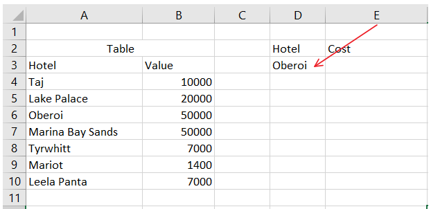
Now we are looking for the cost of the hotel at D3.
So our lookup_value will be D3.

Lookup cell is D3
=VLOOKUP(D3,table,column_index, [range_lookup])
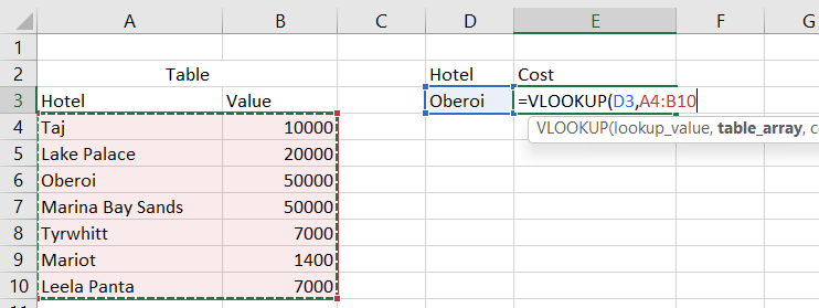
Now our table values start from A4 and end at B10.
Thus the table in the syntax will be replaced by A4:B10, as shown in the figure below.
We select the table, and thus the values A4:B10 will be shown in excel.

Table A4:B10
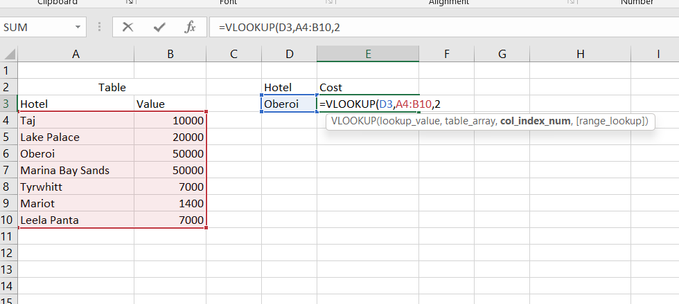
Now we want to retrieve the cost. The hotel names are in the 1st column in the table, and their costs are in the 2nd column. As we want the cost of the hotel, we must supply index 2.

col_index_num will be 2 because the values are in the 2nd column of the table
Now as the [range_lookup], we provide argument FALSE, which represents the exact match.

We then click enter, and the cost of the Oberoi Hotel will be shown in the current cell as shown in the below figure.

We get the cost of the Hotel Oberoi
Dynamic values in the table
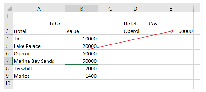
Now, as we change the cost of Oberoi in cell B6, the value will also be automatically updated in cell E3. For example, if we change the value of cell B6 to 60000, the value at E3 will be 60000.

Thus VLOOKUP becomes very helpful when the values are dynamic in the table.
Wildcard Matching
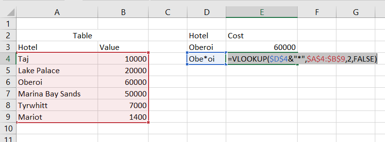
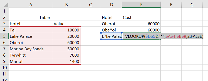
VLOOKUP also supports wildcard matching. Touse wildcard matching for the D4 cell we have to follow the below syntax
=VLOOKUP($D$4&"*",$A$4:$B$9,2,FALSE)
Here we use & “*” which allows the wildcards to be used in the D4.
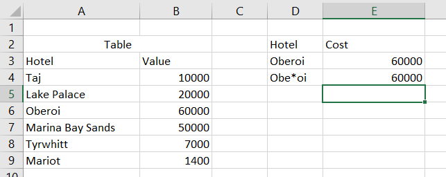
Here * in the word “Obe*oi” represents one or multiple characters in place for *.
Thus “Obe*oi” would match for “Oberoi”, “Oberroi” etc.


Wildcard matching in VLOOKUP
Let us see wildcard matching for “L?ke Oberoi”.
The syntax for this would be
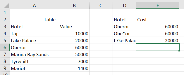
=VLOOKUP($D$5&"*",$A$4:$B$9,2,FALSE)

The output will be 20000 as shown in the below figure.

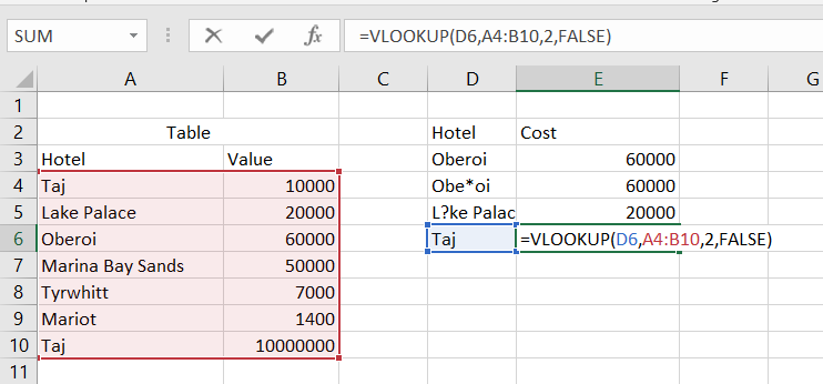
Multiple matches in the table
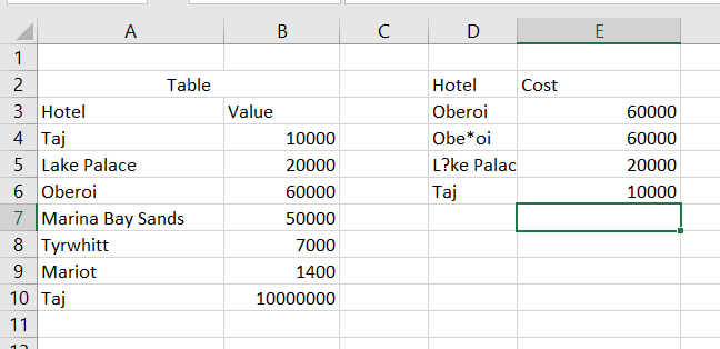
The VLOOKUP returns the first match in case of multiple matches.
For example, in the table, there are two Taj. In this case, the VLOOKUP returns the value of the first appearance of the Taj.

The output will be B4, i.e. 10000

FAQs
1. What is the VLOOKUP function?
VLOOKUP is an Excel function that helps us look up a value in a vertically organised table. It helps us save time.
2. What are the advantages of using the VLOOKUP function?
The advantage of using the VLOOKUP function is that the change in the value of the table will automatically update the output of the VLOOKUP function.
3. What function is similar to VLOOKUP but used for horizontal tables?
The function HLOOKUP is used for lookup when a horizontal table is given. Another function XLOOKUP works for both horizontal and vertical tables.
4. What is the use of wildcard matching in the VLOOKUP?
Using wildcard matching, we can find the lookup values for partial words. For example, we can use Lake * to find a match for Lake Palace.
5. What does the VLOOKUP do when there are multiple matches?
The VLOOKUP function returns the value corresponding to the first matched result.
Key Takeaways
We have extensively discussed the VLOOKUP function in Excel.
We hope that this blog has helped you enhance your knowledge regarding the VLOOKUP function, and if you would like to learn more, check out our articles and archives on cyber security:
Refer to our guided paths on Coding Ninjas Studio to learn more about DSA, Competitive Programming, JavaScript, System Design, etc.
Enrol in our courses and refer to the mock test and problems available.
Take a look at the interview experiences and interview bundle for placement preparations.
Do upvote our blog to help other ninjas grow.
Happy Learning!!!


