HashMaps

Introduction

Suppose we are given a string or a character array and we are asked to find the maximum occurring character. It could be quickly done using arrays. We can simply create an array of size 256, initialize this array to zero, and then, simply traverse the array to increase the count of each character against its ASCII value in the frequency array. In this way, we will be able to figure out the maximum occurring character in the given string.

The above method will work fine for all the 256 characters whose ASCII values are known. But what if we want to store the maximum frequency string out of a  given array of strings? It can’t be done using a simple frequency array, as the strings do not possess any specific identification value like the ASCII values. For this, we will be using a different data structure called hashmaps.

In hashmaps, the data is stored in the form of keys against which some value is assigned. Keys and values don’t need to be of the same data type. 

If we consider the above example in which we were trying to find the maximum occurring string, using hashmaps, the individual strings will be regarded as keys, and the value stored against them will be considered as their respective frequency. 

For example, The given string array is:

str[] = {“abc”, “def”, “ab”, “abc”, “def”, “abc”}

Hashmap will look as follows with strings as keys and frequencies as values : 

From here, we can directly check for the frequency of each string and hence figure out the most frequent string among them all.

Note: One more limitation of arrays is that the indices could only be whole numbers but this limitation does not hold for hashmaps.

The values are stored corresponding to their respective keys and can be invoked using these keys. To insert, we can do the following:

• hashmap[key] = value
• hashmap.insert(key, value)

The functions that are required for the hashmaps are (using templates): 

• insert(k key, v value): To insert the value of type v against the key of type k.
• getValue(k key): To get the value stored against the key of type k.
• deleteKey(k key): To delete the key of type k, and hence the value corresponding to it.

To implement the hashmaps, we can use the following data structures:

1. Linked Lists: To perform insertion, deletion, and search operations in the linked list, the time complexity will be O(n) for each as:
   1. For insertion, we will first have to check if the key already exists or not, if it exists, then we just have to update the value stored corresponding to that key.
   2. For search and deletion, we will be traversing the length of the linked list.
2. BST: We can use some kind of a balanced BST so that the height remains of the order O(logN). For using a BST, we will need some sort of comparison between the keys. In the case of strings, we can do the same. Hence, insertion, search, and deletion operations are directly proportional to the height of the BST. Thus the time complexity reduces to O(logN) for each.
3. Hash table: Using a hash table, the time complexity of insertion, deletion, and search operations, could be improved to O(1) (same as that of arrays). We will study this in further sections.

Bucket array and Hash function

Now, let’s see how to perform insertion, deletion, and search operations using hash tables.  Arrays are one of the fastest ways to extract data as compared to other data structures as the time complexity of accessing the data in the array is O(1), so we will try to use them in implementing the hashmaps.

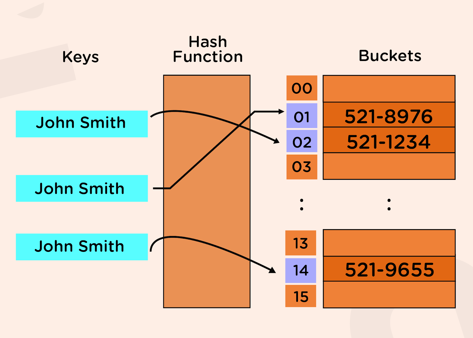
Now, we want to store the key-value pairs in an array, named bucket array. We need an integer corresponding to the key so that we can keep it in the bucket array. To do so, we use a hash function. A hash function converts the key into an integer, which acts as the index for storing the key in the array.

For example: Suppose, we want to store some names from the contact list in the hash table, check out the following image:

Suppose we want to store a string in a hash table, and after passing the string through the hash function, the integer we obtain is equal to 10593, but the bucket array’s size is only 20. So, we can’t store that string in the array as 10593, as this index does not exist in the array of size 20.

To overcome this problem, we will divide the hashmap into two parts:

• Hash code
• Compression function

The first step to store a value into the bucket array is to convert the key into an integer (this could be any integer irrespective of the size of the bucket array). This part is achieved by using a hashcode. For different types of keys, we will be having different kinds of hash codes. Now we will pass this value through the compression function, which will convert that value within the range of our bucket array’s size. Now, we can directly store that key against the index obtained after passing through the compression function.

The compression function can be used as (%bucket_size). 

One example of a hash code could be: (Example input: "abcd") 

"abcd" = ('a' * p^3) + ('b' * p^2) + ('c' * p^1) + ('d' * p^0)

Where p is generally taken as a prime number so that they are well distributed.

But, there is still a possibility that after passing the key through from hash code, when we give the same through the compression function, we can get the same values of indices. For example, let s1 = “ab” and s2 = “cd”. Now using the above hash function for p = 2, h1 = 292 and h2 = 298. Let the bucket size be equal to 2. Now, if we pass the hash codes through the compression function, we will get:

Compression_function1 = 292 % 2 = 0
Compression_function2 = 298 % 2 = 0

This means they both lead to the same index 0.

This is known as a collision.

Collision Handling 

We can handle collisions in two ways:

• Closed hashing (or closed addressing)
• Open addressing

In closed hashing, each entry of the array will be a linked list. This means it should be able to store every value that corresponds to this index. The array position holds the address to the head of the linked list, and we can traverse the linked list by using the head pointer for the same and add the new element at the end of that linked list. This is also known as separate chaining.

On the other hand, in open addressing, we will check for the index in the bucket array if it is empty or not. If it is empty, then we will directly insert the key-value pair over that index. If not, then will we find an alternate position for the same. To find the alternate position, we can use the following:

hi(a) = hf(a) + f(i)

Where hf(a) is the original hash function, and f(i) is the ith try over the hash function to obtain the final position hi(a).

To figure out this f(i), the following are some of the techniques:

1. Linear probing: In this method, we will linearly probe to the next slot until we find the empty index. Here, f(i) = i.
2. Quadratic probing: As the name suggests, we will look for alternate i^2 positions ahead of the filled ones, i.e., f(i) = i^2.
3. Double hashing: According to this method, f(i) = i * H(a), where H(a) is some other hash function.

In practice, we generally prefer to use separate chaining over open addressing, as it is easier to implement and is also more efficient.

Advantages of HashMaps

• Fast random memory access through hash functions
• Can use negative and non-integral values to access the values.
• Keys can be stored in sorted order hence can iterate over the maps easily.

Disadvantages of HashMaps

• Collisions can cause large penalties and can blow up the time complexity to linear.
• When the number of keys is large, a single hash function often causes collisions.

Applications of HashMaps

• These have applications in implementations of Cache where memory locations are mapped to small sets.
• They are used to index tuples in Database management systems.
• They are also used in algorithms like the Rabin Karp pattern matching