Graphs

Introduction to graphs

A graph G is defined as an ordered set (V, E), where V(G) represents the set of vertices, and E(G) represents the edges that connect these vertices.

The vertices x and y of an edge {x, y} are called the endpoints of the edge. The edge is said to join x and y and to be incident on x and y. A vertex may not belong to any edge.

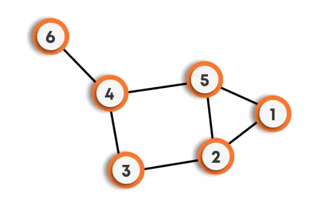
For example: Suppose there is a road network in a country, where we have many cities, and roads are connecting these cities. There could be some cities that are not connected by some other cities like an island. This structure seems to be non-uniform, and hence, we can’t use trees to store it. In such cases, we will be using graphs. Refer to the figure for better understanding.

V(G) = {1,2,3,4,5,6}

E(G) = {(1,2), (1,5), (2,5), (5,4), (2,3), (3,4), (4,6)}

A graph can be undirected or directed.

• Undirected Graphs: In undirected graphs, edges do not have any direction associated with them. In other words, if an edge is drawn between nodes A and B, then the nodes can be traversed from A to B as well as from B to A.
• Directed Graphs: In directed graphs, edges form an ordered pair. In other words, if there is an edge from A to B, then there is a direct path from A to B but not from B to A. The edge (A, B) is said to initiate from node A (also known as an initial node) and terminate at node B (terminal node).

A graph can be weighted or unweighted.

• Unweighted Graphs: In unweighted graphs, an edge does not contain any weight.
• Weighted Graphs: If edges in a graph have weights associated with them, then the graph is said to be weighted.

Relationship between graphs and trees

• A tree is a special type of graph in which we can reach any node from any other node using some path that is unique, unlike the graphs where this condition may or may not hold.
• A tree is an undirected connected graph with N vertices and exactly N-1 edges.
• A tree does not have any cycles in it, while a graph may have cycles.

Graph Terminology

• Nodes are called vertices, and the connections between them are called edges.
• Two vertices are said to be adjacent if there exists a direct edge connecting them.
• The degree of a node is defined as the number of edges that are incident to it. If the degree of vertex u is 0, it means that u does not belong to any edge and such a node is known as an isolated vertex.
• A loop is an edge that connects a vertex to itself.
• Distinct edges that connect the same end-points are called multiple edges.
• A path is a collection of edges through which we can reach from one node to the other node in a graph. A path P is written as P = {v0,v1,v2,....,vn} of length n from a node u to node v, is defined as a sequence of (n+1) nodes. Here u = v0, v = vn and vi-1 is adjacent to vi for i = 1,2,3,.....,n.
• A path in which the first and the last vertices are the same forms a cycle.
• A graph is said to be simple, if it is undirected and unweighted, containing no self-loops and multiple edges.
• A graph with multiple edges and/or self-loops is called a multi-graph.
• A graph is said to be connected if there is a path between every pair of vertices.
• If the graph is not connected, then all the maximally connected subsets of the graphs are called connected components. Each component is connected within itself, but two different components of a graph are never connected.
• The minimum number of edges in a graph can be zero, which means a graph could have no edges as well.
• The minimum number of edges in a connected graph will be (N-1), where N is the number of nodes.
• In a complete graph (where each node is connected to every other node by a direct edge), there are NC2 number of edges means (N * (N-1)) / 2 edges, where N is the number of nodes, this is the maximum number of edges that a simple graph can have.
• Hence, if an algorithm works on the terms of edges, let’s say O(E), where E is the number of edges, then in the worst case, the algorithm will take O(N2) time, where N is the number of nodes.

DIRECTED GRAPHS - 

• The number of edges that originate at a node is the out-degree of that node.
• The number of edges that terminate at a node is the in-degree of that node.
• The degree of a node is the sum of the in-degree and out-degree of the node.
• A digraph or directed graph is said to be strongly connected if and only if there exists a path between every pair of nodes in the graph.
• A digraph is said to be a simple directed graph if and only if it has no parallel edges. However, a simple directed graph may contain cycles with the exception that it cannot have more than one loop at a given node.
• A digraph is said to be a directed acyclic graph(DAG) if the directed graph has no cycles.

Graphs Representation

Suppose the graph is as follows:

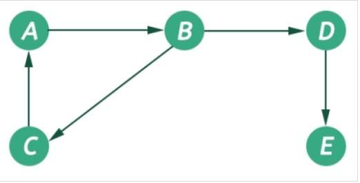
There are the following ways to implement a graph:

• Using edge list: We can create a class that could store an array of edges. The array of edges will contain all the pairs that are connected, all put together in one place. It is not preferred to check for a particular edge connecting two nodes; we have to traverse the complete array leading to O(n2) time complexity in the worst case. Pictorial representation for the above graph using the edge list is given below:
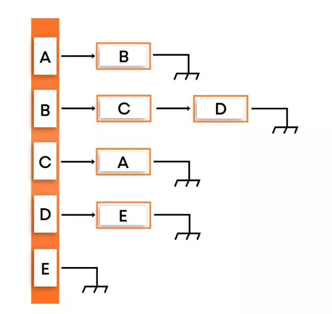
• Adjacency list: We will create an array of vertices, but this time, each vertex will have its list of edges connecting this vertex to another vertex. The key advantages of using an adjacency list are:

1. It is easy to follow and clearly shows the adjacent nodes of a particular node
2. It is often used for storing graphs that have a small-to-moderate number of edges. That is, an adjacency list is preferred for representing sparse graphs in the computer’s memory; otherwise, an adjacency matrix is a good choice.
3. Adding new nodes in G is easy and straightforward when G is represented using an adjacency list.

• Adjacency matrix: Here, we will create a 2D array where the cell (i, j) will denote an edge between node i and node j. The major disadvantage of using the adjacency matrix is vast space consumption compared to the adjacency list, where each node stores only those nodes that are directly connected to them. For the above graph, the adjacency matrix looks as follows:

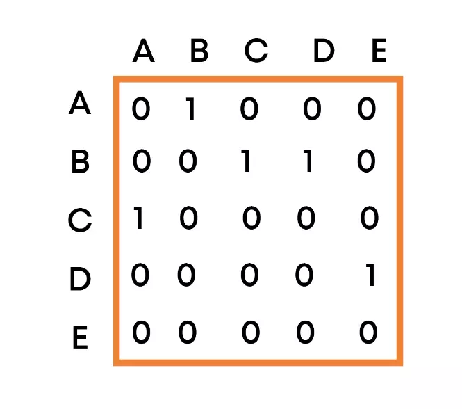
1. For a simple graph (that has no loops), the adjacency matrix has 0s on the diagonal
2. The adjacency matrix of an undirected graph is symmetric.
3. The memory use of an adjacency matrix for n nodes is O(n^2), where n is the number of nodes in the graph.
4. The adjacency matrix for a weighted graph contains the weights of the edges connecting the nodes.

Graph traversal algorithms

Traversing a graph means examining the nodes and edges of the graph. There are two standard methods of graph traversal which we will discuss in this section. These two methods are - 

a) Depth-first search 

b) Breadth-first search.

While breadth-first search uses a queue as an auxiliary data structure to store nodes for further processing, the depth-first search scheme uses a stack. But both these algorithms make use of a bool variable VISITED. During the execution of the algorithm, every node in the graph will have the variable VISITED set to false or true, depending on its current state, whether the node has been processed/visited or not.

Depth-first search (DFS)

The depth-first search(DFS) algorithm, as the name suggests, first goes into the depth and then recursively does the same in other directions, it progresses by expanding the starting node of G and then going deeper and deeper until the goal node is found, or until a node that has no children is encountered. When a dead-end is reached, the algorithm backtracks, returning to the most recent node that has not been completely explored.

In other words, the depth-first search begins at a starting node A which becomes the current node. Then, it examines each node along with a path P which begins at A. That is, we process a neighbor of A, then a neighbor of the processed node, and so on. During the execution of the algorithm, if we reach a path that has a node that has already been processed, then we backtrack to the current node. Otherwise, the unvisited (unprocessed) node becomes the current node.

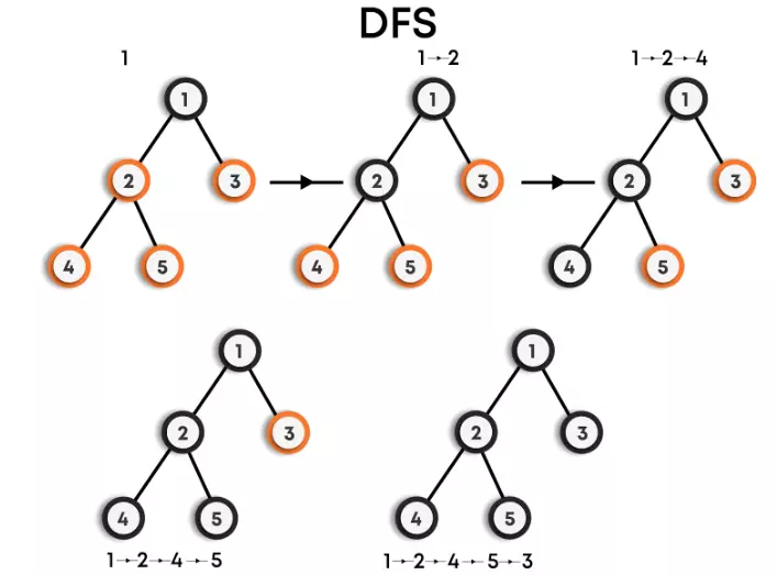
For example: DFS for the below graph is:

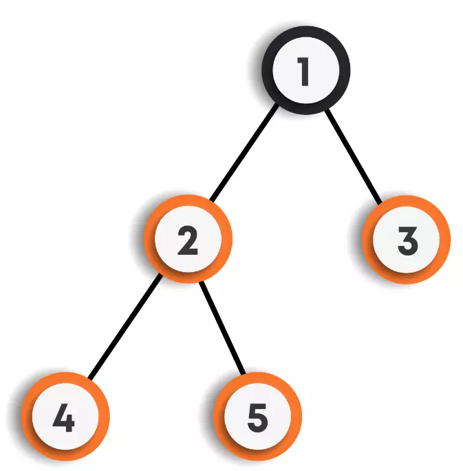
DFS Traversal : 1->2->4->5->3

Other possible DFS traversals for the above graph can be:

1. 1->3->2->4->5
2. 1->2->5->4->3
3. 1->3->2->5->4

We can clearly observe that there can be more than one DFS traversals for the same graph.

Pseudocode(DFS: Iterative)

function DFS_iterative(graph,source)
    
    /*
        Let St be a stack, pushing source vertex in the stack.
        St represents the vertices that have been processed/visited 
        so far.
    */

    St.push(source)
    
    //   Mark source vertex as visited.
    visited[source] = true

    //   Iterate through the vertices present in the stack

    while St is not empty
        //   Pop a vertex from the stack to visit its neighbors
        cur = St.top()
        St.pop()

        /*
            Push all the neighbors of the cur vertex that have not been visited yet, push them into the stack and 
            mark them as visited.
        */

        for all neighbors v of cur in graph:
            if visited[v] is false
                St.push(v)
                visited[v] = true
    
    return

Pseudocode(DFS: Recursive)

function DFS_recursive(graph,cur)

    //   Mark the cur vertex as visited.
    visited[cur] = true

    /* 
        Recur for all the neighbors of the cur vertex that have not been visited yet.
    */

    for all neighbors v of cur in graph:
        if visited[v] is false
            DFS_recursive(graph,v)
    return

Features of Depth-First Search Algorithm

• Time Complexity: The time complexity of a depth-first search is proportional to the number of vertices plus the number of edges in the graphs that are traversed. The time complexity can be given as (O(|V| + |E|)), where |V| is the number of vertices and |E| is the number of edges in the graph considering the graph is represented by adjacency list.
• Completeness: Depth-first search is said to be a complete algorithm in the case of a finite graph. If there is a solution, a depth-first search will find it regardless of the kind of graph. But in the case of an infinite graph, where there is no possible solution, it will diverge.

Applications of Depth-First Search Algorithm

• Finding a path between two specified nodes, u and v, of an unweighted graph.
• Finding a path between two specified nodes, u and v, of a weighted graph.
• Finding whether a graph is connected or not.
• Computing the spanning tree of a connected graph

Breadth-first search (BFS)

Breadth-first search(BFS) is a graph search algorithm where we start from the selected node and traverse the graph level-wise or layer-wise, thus exploring the neighbor nodes (which are directly connected to the starting node), and then moving on to the next level neighbor nodes.

As the name suggests:

• We first move horizontally and visit all the nodes of the current layer.
• Then move to the next layer.

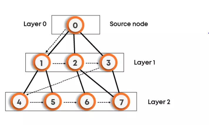
BFS Traversal: 0->1->2->3->4->5->6->7

Other possible BFS traversals for the above graph can be:

1. 0->3->2->1->7->6->5->4
2. 0->1->2->3->5->4->7->6

We can clearly observe that there can be more than one BFS traversals for the same graph, as shown for the above graph.

That is, we start examining say node A and then all the neighbors of A are examined. In the next step, we examine the neighbors of A, so on, and so forth. This means that we need to track the neighbors of the node and guarantee that every node in the graph is processed and no node is processed more than once. This is accomplished by using a queue that will hold the nodes that are waiting for further processing and a variable VISITED to represent the current state of the node.

For example: BFS for the below graph is:

Pseudocode(BFS)

function BFS(graph,source)

    /*
        Let Q be a queue, pushing source vertex in the queue.
        Q represents the vertices that have not been processed or
        visited so far, and their neighbors have not been processed.
    */            

    Q.enqueue(source)
    visited[source] = true

    //   Iterate through the vertices in the queue.
    while Q is not empty
        //   Pop a vertex from the queue to visit its neighbors
        cur = Q.front()
        Q.dequeue()

        /*
            Push all the neighbors of the cur vertex that have not been visited yet, push them into the queue and
            mark them as visited.
        */

        for all neighbors v of cur in graph:
            if visited[v] is false
                Q.enqueue(v)
                visited[v] = true
    
    return

Features of Breadth-First Search Algorithm

• Time Complexity: The time complexity of a breadth-first search is proportional to the number of vertices plus the number of edges in the graphs that are traversed. The time complexity can be given as (O(|V| + |E|)), where |V| is the number of vertices in the graph and |E| is the number of edges in the graph, considering the graph is represented by adjacency list.
• Completeness: Breadth-first search is said to be a complete algorithm in the case of a finite graph because if there is a solution, the breadth-first search will find it regardless of the kind of graph. But in the case of an infinite graph where there is no possible solution, it will diverge.

Applications of Breadth-First Search algorithm

• Finding all connected components in a graph G.
• Finding all nodes within an individual connected component
• Finding the shortest path between two nodes, u and v, of an unweighted graph. (The shortest path is in terms of the minimum number of moves required to visit v from u or vice-versa).

NOTE:

• The DFS and BFS algorithms work for both directed and undirected graphs, weighted and unweighted graphs, connected and disconnected graphs.
• For disconnected graphs, for traversing the whole graph, we need to call DFS/BFS for each unvisited vertex.For getting the number of connected components in a graph, the number of times we need to call DFS/BFS traversal for the graph on an unvisited vertex gives the number of connected components in the graph.

Applications of graphs

Graphs are very powerful data structures, they are very important in modeling data, many problems can be reduced to known graph problems, hence find many applications, some of them are - 

• Social network graphs: Graphs can be modeled to represent social networks to represent who knows whom, who communicates with whom, who influences whom, or other relationships in social structures
• Transportation networks: In road networks vertices are intersections and edges are the road segments between them, and for public transportation networks vertices are stops and edges are the links between them. They are also used for studying traffic patterns, traffic light timings, and many aspects of transportation.
• Document link graphs: The best-known example is the link graph of the web, where each web page is a vertex, and each hyperlink a directed edge. Link graphs are used, for example, to analyze the relevance of web pages, the best sources of information, and good link sites.
• Neural Networks: Vertices represent neurons and edges represent the synapses between them. Neural networks are used to understand how our brain works and how connections change when we learn. The human brain has about 10^11 neurons and close to 10^15 synapses.
• Epidemiology: Vertices represent individuals and directed edges represent the transfer of an infectious disease from one individual to another. Analyzing such graphs has become an important component in understanding and controlling the spread of diseases.
• Scene graphs: In graphics and computer games scene graphs represent the logical or spatial relationships between objects in a scene. Such graphs are very important in the computer games industry.
• Compilers: Graphs are used extensively in compilers. They can be used for type inference, for so-called data flow analysis, register allocation, and many other purposes. They are also used in specialized compilers, such as query optimization in database languages.
• Dependence graphs: Graphs can be used to represent dependencies or precedences among items. Such graphs are often used in large projects in laying out what components rely on other components and used to minimize the total time or cost to completion while abiding by the dependencies.
• Robot planning: Vertices represent states the robot can be in and the edges the possible transitions between the states. Such graph plans are used, for example, in planning paths for autonomous vehicles.