


Problem
Submissions
Hints & solutions
Discuss
Round Robin Scheduling
Easy

0/40
Average time to solve is 15m
Contributed by
8 upvotes
Asked in companies

Problem statement
In an operating system, processes are scheduled to execute using many algorithms, of which one is the Round Robin Algorithm. This algorithm ensures democracy in utilizing the CPU time for each of the processes currently in execution.
Each process can leave this execution loop when its own execution time is over. Therefore, the process with the largest execution time will be the one that would be the last process waiting. Simulate the Round Robin algorithm execution using the set of process burst times and process ids are given.
The processes (runtime) are to be inserted into the queue first and then decremented (by CPU execution time) for each iteration through the queue until their runtime is over.
For ExampleInput:
# Process id's
proc = [1, 2, 3]
n = 3
# Burst time of all processes
burst_time = [10, 5, 8]
# Time quantum
quantum = 2;
Output:
Processes Burst time Waiting time Turnaround time
1 10 13 23
2 5 10 15
3 8 13 21
Average waiting time = 12
Average turnaround time = 19.6667
Detailed explanation ( Input/output format, Notes, Images )
Input Format:
The first line of input is the number of  test cases ‘T’ which are going to be there

The first line of each test case would be two space-separated integers majorly representing the  ‘numberOfProcesses’ and ‘timeQuanta’.

The second line of each test case contains 'numberOfProcesses' space-separated integers denoting the elements of the array processes.

The third line of each test case contains 'numberOfProcesses' space-separated integers denoting the burst-times of the processes given.
For every test case, print the average wait time and turn around time for the calculated set of processes given the round-robin strategy which is to be used. Print the closest integer less than or equal to a given number.
You do not need to print anything, it has already been taken care of. Just implement the given function.
1 <= T <= 5
1 <= process.length <= 10^5
1 <= processId <= process.length
1 <= burstTimes.length <= process.length
1 <= burstTimes <= 10^5
1 <= timeQuantum <= burst times

Where ‘process.length’ would denote the number of process id which would be given the schedule using the round-robin algorithm, where ‘burstTimes’ are the running times of the given processes (CPU execution times) while the “timeQuantum” is the time duration (slot).

Time Limit: 1 sec
Sample Input 1:
2
4 4
1 2 3 4
5 3 8 9
3 1
1 2 3
3 4 3
Sample Output 1:
10 17
5 8
Explanation For Sample Input 1:
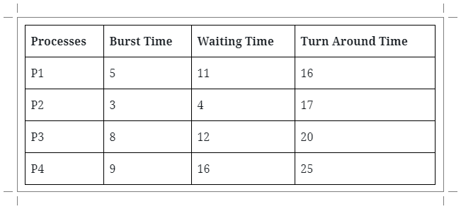
Average Waiting time = ( 11 + 4 + 12 + 16 ) / 4 = 10
Average Turnaround Time = ( 16 + 7 + 20 + 25 ) / 4 = 17

Average waiting time = ( 4 + 6 + 6 ) / 3 = 5
Average Turnaround time = ( 7 + 10 + 9 ) / 3 = 8
Sample Input 2:
1
3 2
1 2 3
10 5 8
Sample Output 2:
12 19
Explanation For Sample Input 2:

Average Waiting time = ( 13 + 10 + 13 ) / 3 = 12
Average Turnaround Time = ( 23 + 15 + 21 ) / 3 = 19
Hint
Hint 1
Can you design an algorithm to calculate the waiting time first and then the turnaround time?
Approaches (1)
Approach 1
Constructive Algorithm
Approach: The tricky part is to compute waiting times. Once waiting times are computed, turn around times can be quickly calculated.
The required terms used here are as follows:
Completion Time: Time at which process completes its execution.
Turn Around Time: Time Difference between completion time and arrival time.
Turn Around Time = Completion Time – Arrival Time
Waiting Time(W.T.): Time Difference between turn around time and burst time.
Waiting Time = Turnaround Time – Burst Time
The algorithm to calculate waiting time and turnaround times will be-
- Create a list (array) ‘REM_BT’ to keep track of remaining burst time of processes. This list is initially a copy of the ‘BT’ (burst times list)
- Create another list (array) ‘WT’ to store waiting times of processes. Initialize this list (array) as 0.
- Initialize time 'T' as 0.
- Keep traversing all processes while all processes are not done. Do the following for ‘i’ th process if it is not done yet.
- If ‘REM_BT[i]’ > ‘QUANTUM’:
- Then increment ‘T’ by ‘QUANTUM’.
- Decrement ‘REM_BT[i]’ by ‘QUANTUM’.
- Else it is last cycle for this process.
- Then increment ‘T’ by ‘QUANTUM’.
- Assign the value of ‘T’ - ‘BT[i]’ to ‘WT[i]’.
- Assign the value 0 to ‘REM_WT[i]’.
- If ‘REM_BT[i]’ > ‘QUANTUM’:
5. Once we have waiting times, we can compute turn around time ‘TAT[i]’ of a process as sum of waiting and burst times, i.e., ‘WT[i] + BT[i]’.
6. We finally return the average waiting time and average turnaround time.
Time Complexity
O(N), where ‘N’ is the total number of processes required to be processed.
Since, for the process, we traverse the list of processes and keep wait times and turn around times for processes in each iteration, hence, the time complexity grows by O(N).
Space Complexity
O(N), where ‘N’ is the total number of processes required to be processed.
We are using a waiting times list (array) and turnaround times to store the required values hence, the Space Complexity is O( N ).
Code Solution
(100% EXP penalty)
Round Robin Scheduling
C++ (g++ 5.4)
Console