


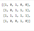
The area of the largest square submatrix with all 1s is 4.
The first line contains an integer ‘T’ denoting the number of test cases. Then each test case follows.

The first input line of each test case contains two space-integers ‘N’ and ‘M’ representing the number of rows and columns of the grid, respectively.

From the second line of each test case, the next N lines represent the rows of the grid. Every row contains M single space-separated integers.
For each test case, print the area of maximum size square sub-matrix with all 1s.

Print the output of each test case in a separate line.
You are not required to print the expected output; it has already been taken care of. Just implement the function.
1 <= T <= 100
1 <= N <= 50
1 <= M <= 50
0 <= MAT[i][j] <= 1

Time limit: 1 sec
We will check for each length of the square that can be possible in the grid. The maximum length of the square that can be possible in the grid is min(N, M).
We will use the prefix sum of the grid to calculate the sum of elements of a submatrix in constant time.
We know the minimum and maximum limit of the side length of the square. So, we will apply binary search to the range of length, instead of checking for each length.
The idea behind using binary search is that if there exists a square of length ‘x’ with all 1s then it is guaranteed that there exist squares with lengths 1 to x - 1.
We will again use the prefix sum of the matrix to find the sum of any submatrix of the grid in constant time.
We will use dynamic programming where MAT[i][j] represents the side length of the maximum square whose bottom right corner is the cell with index (i, j).
We traverse the whole grid and when MAT[i][j] == 0, then no square will be able to contain this cell. If MAT[i][j] == 1, we will have MAT[i][j] = 1 + min(MAT[i-1][j], MAT[i][j-1], MAT[i-1][j-1]), which means that the square will be limited by its left, upper and upper-left neighbors.
Here is the algorithm:
Count of Subsequences with Given Sum
Optimal Line Arrangement
Distinct Integers After Zero Removal
Maximize Partition Value
Maximum Value Path in a Graph

