


The first line contains an integer 'T' which denotes the number of test cases or queries to be run. Then the test cases follow.

The first line of each test case contains two single space-separated integers N and M, denoting the number of rows and columns respectively.

The next 'N' lines, each contains 'M' single space-separated integers representing the elements in a row of the matrix.
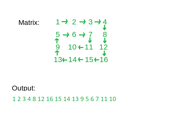
For each test case/query, print the spiral path of the given matrix.

Output for every test case will be printed in a separate line.
You do not need to print anything, it has already been taken care of. Just implement the given function.
1 <= T <= 10
1 <= N <= 100
1 <= M <= 100
-10^9 <= data <= 10^9

where ‘T’ is the number of test cases,  ‘N’ and ‘M’ are the numbers of rows and columns respectively and ‘data’ is the value of the elements of the matrix.
For each boundary, we will use the 4 loops. Now the problem is reduced to print the remaining submatrix which is handled with the help of recursion. Keep track of new dimensions(rows and columns) of the current submatrix which are passed with the help of parameters in each recursion call.
Algorithm:
spiralPrint(matrix[][], startingRow, startingCol, endingRow, endingCol):
The idea is to traverse the matrix using loops where each loop will be used for a specific direction to print all the elements in the clockwise order layer by layer. Every loop traverses the matrix in a single direction. The first loop traverses the matrix from left to right, the second loop traverses the matrix from top to bottom, the third traverses the matrix from the right to left, and the fourth traverses the matrix from bottom to up. After completing the traversal using 4 loops one time, repeat it again for the remaining submatrix. To traverse using these loops we will initialize 4 variables to keep the boundaries of the submatrix as explained below.
Algorithm:
spiralPrint(matrix[][], rows, cols):
In previous approaches, we are using four loops to print the boundary of a matrix.
For this, we will take four operations { (0,1), (1,0), (0,-1), (-1,0) } which will change row or column. We will iterate on these operations cyclically, i.e, operation 1 is next to operation 4.
We will make a 2D array to store the visited cells.
Take two variables R (current row) and C (current column) and initialize them with 0. Let’s take another variable ‘cur’ which denotes the type operation to be performed, initially it will be 0.
Algorithm:
Run a loop from 1 to total number of elements in the matrix:

