


Introduction
Besides solving coding problems, one should be aware of the time complexity of the implemented algorithm so that it can be optimized further.
As a programmer, when trying to solve a problem and create an algorithm for the problem, you must remember that there can be multiple solutions for that particular, depending on the approach.
So if there are many solutions to a problem in the world of programming, then how to decide which solution is good or not? Well, that depends on the application's requirements, like whether the application should be efficient in terms of space or time. Space and time are the two most important factors in judging the efficiency of a program or algorithm. To learn more about space and time complexity, you can go to time complexity as well as space complexity.
This blog will discuss two problem statements to showcase the time complexity. But before we look into the problems, we need to understand time complexity.
Time Complexity
Time complexity is the concept we use to analyze the time taken by an algorithm or program with respect to the input size. Remember that the time complexity is not the actual time taken by the program to generate the output; it is a theoretical concept that gives us an idea of how efficient the algorithm is with respect to the input size.
The actual running time of an algorithm or program depends on various factors like the machine's computational power. We cannot generate the running time of the algorithm.
To solve this problem, we use the concept of time complexity to get a rough estimate of the time with respect to the input of a program. Our goal is to write an efficient program in terms of time when we provide large data as input to the program.
To judge the algorithm's efficiency, we can classify it into the following area depending on the algorithm's approach. Any algorithm can be classified into some type based on its complexity. See the classes mentioned below. We will talk about the Big-O time complexities because it is the average worst time taken which is considered an excellent way to judge an algorithm's efficiency.
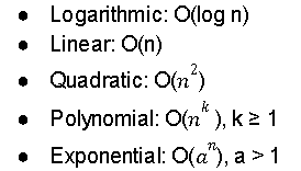
Here n is the size of the input, a is the exponent integer, and k is the degree of n.
Let's see the graphical representation of the above complexities and observe how each of them behaves for a particular input size.

Before we talk about the representation, let's see what each color of the line in the graph represents. You can see the line color on the left side of the complexity.

On the x-axis, we are measuring the user input, and on the y-axis time complexity. From all the lines, we can observe that the blue line gives us linear time as we go further on the x-axis concerning the y-axis.
The large input size does not significantly affect the blue line, which is Logarithmic: O(log n) time. As you can see, the rest of the lines increase significantly as the input size increases for the blue line. This shows that the logarithmic time complexity is the best average time to process the input.
To learn more about Big-O notation, check out the below video.
Now that we have understood the basics of time complexity let's analyze the time complexity question.
Also see, Euclid GCD Algorithm


 18+ registered

