Machine learning With Scikit-learn and XGBoost

Introduction

Scikit-learn began as "scikits.learn", a Google Summer of Code project. It gets its name from being a "SciKit" (SciPy Toolkit), a third-party expansion to SciPy that is created and delivered separately. XGBoost is a scalable and highly accurate gradient boosting implementation that pushes the limits of processing power for boosted tree algorithms. It was designed primarily to energise  Machine Learning model performance and computational speed.

Scikit-learn and XGBoost

Scikit-learn is primarily written in Python and heavily relies on NumPy for high-performance linear algebra and array operations. As we know, Scikit-learn and XGBoost can produce more significant results with lesser work. Extreme Gradient Boosting is abbreviated as XGBoost. The "eXtreme" part of XGBoost's name relates to speed improvements such as parallel processing and cache awareness, which make it around ten times quicker than conventional gradient boosting. XGBoost has an original split-finding algorithm for optimising trees and integrated regularisation to lessen overfitting. In general, XGBoost is a faster, more precise variation of gradient boosting.

Stages of Workflow

We can view the machine learning workflow through the simplified lens of three stages, Preprocessing, Training and Prediction.

Preprocessing

In the preprocessing phase of machine learning, unstructured data is prepared for modelling. It brings us to the term "train", which refers to fine-tuning a model to forecast a target variable using labelled input data. The process of anticipating outcomes for fresh, unlabeled data is called prediction.

Training

The training phase of an ML workflow is the second step. Virtual machines have become much more critical in the modern day. Using the compute engine, we can set up devices with up to four terabytes of RAM. We should be conscious that we are referring to four terabytes of RAM (Random Access Memory) in this case rather than disk space. It even has the computing power to work in tandem with it. So, memory can be put to use. On the software front, libraries like ‘Dask’ enable us to operate with Pandas in parallel without building up a cluster of various PCs. 

Prediction

The Cloud ML Engine is the last component. The Cloud ML Engine can be helpful if our service depends on prediction or if we frequently need to maintain our model on new data. In addition to TensorFlow, Scikit-learn and XGBoost are supported as well. Both training and prediction get served by it. Therefore, we do not need to employ various machine learning libraries with multiple workflows.

Advantages

This library is regarded as one of the best options for machine learning applications, especially in production systems. These include the following but are not limited to them.

• It is an extraordinarily sturdy tool because of the high level of support and strong governance for the development of the library.
• The entry barrier for developing machine learning models is significantly lowered by using a clear, uniform code style that makes the code easy to understand and reproducible.
• It is widely supported by third-party tools, making it feasible to enhance the functionality to meet a variety of use cases.
• The best library to start with while learning machine learning is undoubtedly Scikit-learn. Due to its simplicity, it is relatively simple to learn. Using it, we will also understand the crucial processes in a regular machine learning workflow.

Dataset

The dataset includes crucial characteristics that the model will use while being trained.
This data is used to decide whether or not a person will sign up for a term deposit. If there is additional data in the dataset: Before using the dataset for training and predictive analysis, it must be cleaned.

Packages for Data Analysis (EDA)

We will load the tools we need to analyse and manipulate the data.

Our dataset will be loaded and cleaned using Pandas. For calculations in mathematics and science, Numpy will be used.

import pandas as pd
import numpy as np

Loading Dataset

Let us use Pandas to load the dataset:

df = pd.read_csv("bank-additional-full.csv", sep=";")

The dataset's field separator is set to sep=";".

This is because our dataset's fields are separated by; rather than by its standard separator.

Run this code to see our dataset's structure:

df.head()

Let us look at the data points that are there in our dataset.

df.shape

The result is as follows:

Our dataset comprises 41188 data points and 21 columns, according to the output.

Let us examine these columns:

df.columns

The following picture displays the results:

We will use age, employment, marital status, education, and housing columns to train our model. In the output above, the target variable is the y column. We are attempting to predict this. Either yes or no is written in the y column. If the answer is yes, the customer will subscribe to the term deposit; if the answer is no, the customer will not.

Let us begin clearing our dataset. To begin, we look for missing data.

Checking Missing Data

To check for missing values, we run the following command:

df.isnull().sum()

The findings reveal that there are no missing values in our dataset.

Checking for data types in columns is another step in cleaning up a dataset, as demonstrated below:

The image above has various data types, including object, float64, and int64. Remember that the object data types' values take the form of categories.

These categorical data do not lend themselves to machine learning. To obtain numerical values, we must translate these category values. All data types will be converted to int64. Because the float64 datatype already has a numeric value, we do not need to transform it. Category encoding is the process of transforming categorical values into numeric ones.

Categorical Encoding

Let us obtain all columns that have the object datatype first.

"object" in df.columns[df.dtypes]

The result is displayed:

With the help of the get_dummies() method, we can turn every column into a number.

Categorical data can be transformed into numerical values in a machine-readable format using the Pandas method get_dummies().

when pd.get_dummies(df,df.columns[df.dtypes == 'object']) is used.

The example will produce a new dataset with encoded numeric values:

When we look at the initial lines datasets, we can see that they contain encoded numerical values.

Let us see if the data types for the column have changed.

df.dtypes

The results are displayed in the chart below:

It shows that objects in the columns got changed into an int. Now we may begin creating our model.

This section will use a fundamental Scikit-learn approach to build our model. The performance of the model will then be enhanced using XGBoost.

Installing XGBoost

Let us use this command to install XGBoost:

!pip set up xgboost
Import this package now.
import xgb as xgboost

After importing XGBoost, divide our dataset into training and testing sets.

Dataset Splitting

To split the dataset, we must import train_test_split.

import train_test_split from sklearn.model_selection, 

A training set and a testing set got created from the dataset. 20% of the dataset will be used for testing, while the remaining 80% will be used as a training set.

X_train, X_test, y_train, y_test = train_test_split(X, y, test_size = 0.2, random_state = 0)

We must contrast XGBoost with another algorithm to comprehend its strength.

The decision tree classifier algorithm is first used to construct the model.

Then, using XGBoost to create the same model, we compare the output to determine whether XGBoost has enhanced the model's performance.

Using a decision tree classifier will be our first step.

Decision Tree Classifier

A machine learning algorithm for resolving classification issues is a decision tree classifier. It is a Scikit-learn library import.

When creating a decision rule, branches of the decision tree get employed for strategic analysis.

Decision trees build a model using the input data that predicts the value of the labelled variable.

The distinctive characteristics of a particular dataset are represented by the internal nodes of the tree while creating a model.

Each tree leaf node represents the prediction outcome, while its branches reflect the decision rules.

The chart below shows this:

from sklearn.tree import DecisionTreeClassifier

Let us start the DecisionTreeClassifier from scratch.

dTree_clf = DecisionTreeClassifier()

We can now use the DecisionTreeClassifier to construct our model after initialising it.

Building Model

Our model was adjusted to meet the training set. As a result, the model can recognise and pick up on patterns. In terms of predictive analysis, this is crucial.

dTree_clf.fit(X_train,y_train)

Let us evaluate this model.

Testing Model

Using the test dataset, we evaluate the model. It enables us to assess the model's effectiveness following the training stage.

y_pred2 = dTree_clf.predict(X_test)

Use the following command to view the predictions:

y_pred2

The result is as follows:

The first number in array(1) has a favourable forecast from the model. It demonstrates that someone will sign up for a term deposit with the bank. A few data points' predictions are displayed in this report.

 

Let us determine how accurate these predictions were:

print("Accuracy of Model::",accuracy_score(y_test,y_pred2))

The result is as follows:

It demonstrates that the model has a prediction accuracy score of 89.29%. Let us see if XGBoost can enhance this model's functionality and raise the accuracy rating.

XGBoost

To begin with, we must initialise XGBoost. As previously said, XGBoost builds the best model from other weak models.

Combining many models speeds up the process of identifying and fixing prediction flaws.

XGBoost can raise the model's accuracy score by utilising the most accurate parameters during prediction.

xgb_classifier = xgb.XGBClassifier()

We can use XGBoost to train our model once it gets initialised.

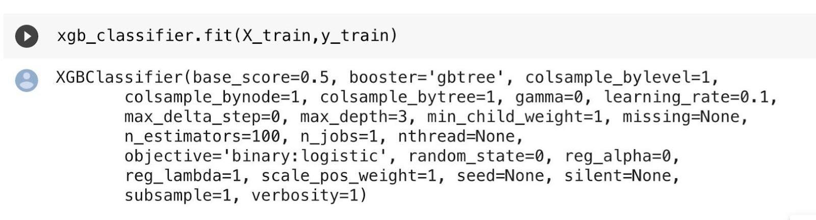
xgb_classifier.fit(X_train,y_train)

We apply the training set once more. The model absorbs knowledge from this dataset, retains it in memory, and applies it to its prediction process.

xgb_classifier.fit(X_train,y_train)

The result is as follows: 

Let us put this model to the test and generate a forecast.

It will put our model to the test to see how effectively it picked up new information during training.

Making Predictions

predictions = xgb_classifier.predict(X_test)

Use this command to see the outcomes of the prediction:

predictions

The result is as follows:

This prediction indicates that the array's initial value will be 0. It is not the decision tree classifier's predicted outcome.

It demonstrates that the prediction error got fixed using XGBoost, resulting in accurate predictions.

 

Let us see if the accuracy rating has improved.

print("Accuracy of Model::",accuracy_score(y_test,predictions))

The accuracy rating is as follows:

It demonstrates that the model has a 92.255 per cent accuracy rating. It represents a higher accuracy score than the decision tree classier's 89.29% accuracy score.