


Introduction
Before going on to the measures of dispersion let us briefly discuss numerical data. Numerical data refers to the data that is available in the form of numbers. The data types of numerical data are integer, floating-point numbers, complex numbers, etc. Examples of numerical data; age, weight, height, etc.
Measures of dispersion are the statistical methods to calculate the spread of the data. It gives information on how far the data points are distributed in the dataset. It captures the variation between different data points. It measures the extent to which data points of the distribution differ from the mean of the distribution.
A major measure of dispersion is; standard deviation, variance, range, interquartile range(IQR), skewness, etc. Let us understand each term in detail.
Standard deviation
It gives the measure of the spread of data points about the mean value of the numerical data. It is also the square root of the variance (𝞂2). If the standard deviation of the dataset is low, then the value of data points is close to the mean.
The formula for standard deviation:
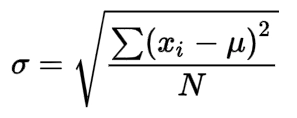
- xi datapoints (1 ≤ i ≤ N)
- N = size of dataset
- u = mean(average)
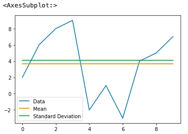
Let us plot the standard deviation using a sample dataset.
|
# importing libraries import pandas as pd import statistics as st import numpy as np from matplotlib import pyplot as plt # creating dataframe data = pd.DataFrame({ "Data": [2, 6, 8, 9, -2, 1, -3, 4, 5, 7] }) # calculating mean and standard deviation SD = data.std() Mean = data.mean() SD, Mean |
|
(Data 4.110961 dtype: float64, Data 3.7 dtype: float64) |
Plotting the data
|
# adding the column of mean data["Mean"] = [float(Mean) for i in range(len(data))] # adding the column of Standard deviation data["Standard Deviation"] = [float(SD) for i in range(len(data))] data.plot() |
Variance
It is a square of standard deviation and also a covariance of a random variable with itself. It is denoted by symbol 𝞂2. If the variance is large, it interprets that the dataset has a higher degree of spread.
The formula for calculating variance is:

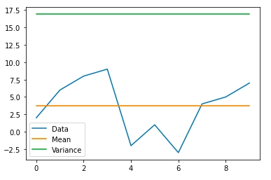
Let us plot the Variance using a sample dataset(same data used for plotting (Standard deviation).
|
# calculating variance var = data["Data"].var() # printing variance print("Variance is",var) # adding column for variance data["Variance"] = [float(var) for i in range(len(data))] # Removing the column of Standard Deviation data = data.drop(['Standard Deviation'], axis = 1) # plotting the data data.plot() |
| Variance is 16.9 |
Range
The range is the difference between the upper and lower bound of the dataset.
| data["Data"].max() - data["Data"].min() |
| 12 |
Interquartile range(IQR)
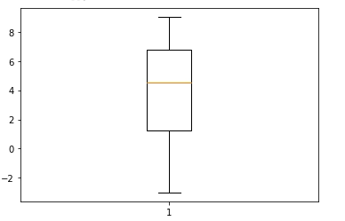
The interquartile range is another statistical measure of dispersion used to calculate spread in numerical data. It is the difference between the upper quartile(75 percentile) and the lower quartile(25 percentile). It is very helpful in identifying outliers. It is visualized using a boxplot.
We are importing the IQR function from the scipy library.
|
from scipy.stats import iqr iqr(data["Data"]) |
| 5.5 |
| plt.boxplot(data["Data"]) |
Skewness
Skewness measures the deviation of the distribution of random variables from a normal distribution. The skewness is important to measure the asymmetricity of the dataset. The values of skewness can be positive, negative, or undefined.
Skewness values can be interpreted in the following way:
- If the skewness value is less than -1 and greater than +1, the data has a highly skewed distribution.
- If the value is skewness between -1 to -½ or between ½ to 1, the data has a moderately skewed distribution.
- If the skewness value is between -½ to ½, the data has an approximately symmetric distribution.
Skewness value can be calculated using the following code:
|
from scipy.stats import skew skew(data["Data"]) -0.3908359884691249 |
Mean Deviation
It calculates the average deviation of the dataset from the mean value. In simple words, it gives us the information of how far the data points are from the dataset's center point. It is variability as compared to standard deviation.
The formula for mean deviation:
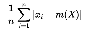
Here m(X) is mean, xi is a data point (1 ≤ i ≤ N).
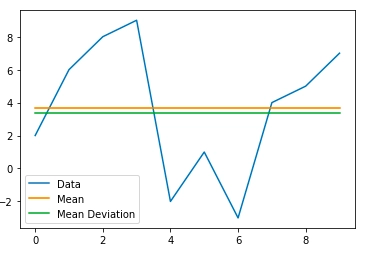
Let us understand the mean deviation using a sample dataset.
|
# getting value of mean deviation md = data["Data"].mad() # adding the mean deviation column data["Mean Deviation"] = [md for i in range(len(data))] # removing the variance column from the previous implementation data = data.drop(['Variance'], axis = 1) # plotting the graph data.plot() |
FAQs
-
What do you mean by measures of dispersion?
The measure of dispersion shows the spread of data. It explains the data differs from one another, delivering a precise picture of the data distribution.
-
What are the uses of measures of dispersion?
Measures of dispersion are used to explain the range of the data, os its variation around the mean
-
What is the best measure of dispersion?
The best measure of dispersion is Standard Deviation; also, it is the most reliable measure of dispersion. Standard deviation helps to compare the variability of two or more sets of data, testing the significance of random samples and in regression and correlation analysis.
-
What are 4 commonly used measures of dispersion?
4 Commonly Used Measures of Dispersion:
Range
Interquartile range
Average Deviation (A.D.) or Mean Deviation (M.D.)
Standard Deviation or S.D. and Variance
-
Why do we measure dispersion?
While measures of central tendency are used to estimate "normal" values of a dataset, measures of dispersion are important for describing the spread of the data, or its variation around a central value.
Key Takeaways
In this article, we have discussed:
- Use of measures of dispersion.
- Standard deviation, variance, range, interquartile range, skewness, mean deviation.
- Implementation of all the measures of dispersion.
Want to learn more about Machine Learning? Here is an excellent course that can guide you in learning.
Happy Coding!

 8+ registered

