Introduction
In the previous blog we defined the generator and the discriminator models now it's time to train those models. If you haven't read that article the link for part 1 is here.
Now we'll see the training part of the generator models in this blog.
Training Progressive Growing GAN Model
Loading Dataset
def load_real_samples(filename):
	data = load(filename)
	# extracting numpy array
	X = data['arr_0']
	# converting from ints to floats
	X = X.astype('float32')
	# scaling from [0,255] to [-1,1]
	X = (X - 127.5) / 127.5
	return X
The next step is to retrieve a random sample of photos for updating the discriminator.
# selecting real samples
def generate_real_samples(dataset, n_samples):
	# choosing random instances
	ix = randint(0, dataset.shape[0], n_samples)
	# selecting images
	X = dataset[ix]
	# generating class labels
	y = ones((n_samples, 1))
return X, yNext, we'll need a sample of latent points to use with the generator model to build synthetic images.
# generating points in latent space as input for the generator
def generate_latent_points(latent_dim, n_samples):
	# generating points in the latent space
	x_input = randn(latent_dim * n_samples)
	# reshaping into a batch of inputs for the network
	x_input = x_input.reshape(n_samples, latent_dim)
return x_inputThe generate fake samples() function takes a generator model returns a batch of synthetic images. The class for all the generated images will be -1 to indicate that they are fake.
# generating points in latent space as input for the generator
def generate_latent_points(latent_dim, n_samples):
	# generating points in the latent space
	x_input = randn(latent_dim * n_samples)
	# reshaping into a batch of inputs for the network
	x_input = x_input.reshape(n_samples, latent_dim)
return x_inputThe models are trained in two phases: a fade-in phase in which the transition from a lower-resolution to a higher-resolution image is made, and a normal phase in which the models are fine-tuned at a given higher resolution image.
# updating the alpha value on each instance of WeightedSum
def update_fadein(models, step, n_steps):
	# calculating current alpha (linear from 0 to 1)
	alpha = step / float(n_steps - 1)
	# updating the alpha for each model
 	for m in models:
  		for layer in m.layers:
    		if isinstance(layer, WeightedSum):
backend.set_value(layer.alpha, alpha)The technique for training the models for a certain training phase can then be defined.
One generator, discriminator, and composite model are updated on the dataset for a fixed number of training epochs during the training phase. The training phase could be a fade-in transition to a higher resolution, in which case update_fadein() must be called each iteration, or a standard tuning training phase, in which case no WeightedSum layers are present.
# training a generator and discriminator
def train_epochs(g_model, d_model, gan_model, dataset, n_epochs, n_batch, fadein=False):
	# calculating the number of batches per training epoch
	bpe = int(dataset.shape[0] / n_batch)
	# calculating the number of training iterations
	ns = bpe * n_epochs
	# calculating the size of half a batch of samples
	hb = int(n_batch / 2)
	# manually enumerating epochs
 	for x in range(ns):
  		# updating alpha for all WeightedSum layers when fading in new blocks
  		if fadein:
    		update_fadein([g_model, d_model, gan_model], x, ns)
  		# preparing real and fake samples
  		X_real, y_real = generate_real_samples(dataset, hb)
  		X_fake, y_fake = generate_fake_samples(g_model, latent_dim, hb)
  		# updating discriminator model
  		d_loss1 = d_model.train_on_batch(X_real, y_real)
  		d_loss2 = d_model.train_on_batch(X_fake, y_fake)
  		# updating the generator via the discriminator's error
  		z_input = generate_latent_points(latent_dim, n_batch)
  		y_real2 = ones((n_batch, 1))
  		g_loss = gan_model.train_on_batch(z_input, y_real2)
  		# summarizing loss on this batch
print('>%d, d1=%.3f, d2=%.3f g=%.3f' % (x+1, d_loss1, d_loss2, g_loss))For each training phase, we must then call the train epochs() function.
Scaling the training dataset to the appropriate pixel dimensions, such as 44 or 88, is the first step. This is accomplished via the scale_dataset() function, which takes a dataset and returns a scaled version.
# scaling images to preferred size
def scale_dataset(images, new_shape):
	images_list = list()
 	for image in images:
  		# resizing with nearest neighbor interpolation
  		new_image = resize(image, new_shape, 0)
  		# storing
  		images_list.append(new_image)
return asarray(images_list)We also need to preserve a plot of generated images and the current state of the generator model after each training run.
# generating samples and saving as a plot and saving the model
def summarize_performance(status, g_model, latent_dim, n_samples=25):
	# devising a name
	gs = g_model.output_shape
	nm = '%03dx%03d-%s' % (gs[1], gs[2], status)
	# generating images
	X, _ = generate_fake_samples(g_model, latent_dim, n_samples)
	# normalizing pixel values to the range [0,1]
	X = (X - X.min()) / (X.max() - X.min())
	# plotting real images
	square = int(sqrt(n_samples))
	for i in range(n_samples):
  		pyplot.subplot(square, square, 1 + i)
  		pyplot.axis('off')
  		pyplot.imshow(X[i])
	# saving a plot to file
	f1 = 'plot_%s.png' % (nm)
	pyplot.savefig(f1)
	pyplot.close()
	# saving the generator model
	f2 = 'model_%s.h5' % (nm)
	g_model.save(f2)
print('>Saved: %s and %s' % (f1, f2))The train() function takes the lists of defined models, as well as the list of batch sizes and the number of training epochs for the normal and fade-in phases for each degree of growth for the model, as inputs.
# training the generator and discriminator
def train(g_models, d_models, gan_models, dataset, latent_dim, e_norm, e_fadein, n_batch):
	# fitting the baseline model
	gn, dn, gan_n = g_models[0][0], d_models[0][0], gan_models[0][0]
	# scaling dataset to appropriate size
	gs = gn.output_shape
	sd = scale_dataset(dataset, gs[1:])
	print('Scaled Data', sd.shape)
	# training normal or straight-through models
	train_epochs(gn, dn, gan_n, sd, e_norm[0], n_batch[0])
	summarize_performance('tuned', gn, latent_dim)
	# processing each level of growth
	for i in range(1, len(g_models)):
  		# retrieving models for this level of growth
  		[gn, g_fadein] = g_models[i]
  		[dn, d_fadein] = d_models[i]
  		[gan_n, gan_fadein] = gan_models[i]
  		# scaling the dataset to appropriate size
  		gs = gn.output_shape
  		sd = scale_dataset(dataset, gs[1:])
  		print('Scaled Data', sd.shape)
  		# training fade-in models for next level of growth
  		train_epochs(g_fadein, d_fadein, gan_fadein, sd, e_fadein[i], n_batch[i], True)
  		summarize_performance('faded', g_fadein, latent_dim)
  		# training normal or straight-through models
  		train_epochs(gn, dn, gan_n, sd, e_norm[i], n_batch[i])
summarize_performance('tuned', g_normal, latent_dim)Finally, let us call the defined models, and call train() function to start the training process.
# number of growth phases, e.g. 6 == [4, 8, 16, 32, 64, 128]
n_blocks = 6
# size of the latent space
latent_dim = 100
# defining models
dm = define_discriminator(n_blocks)
# defining models
gm = define_generator(latent_dim, n_blocks)
# defining composite models
gan_m = define_composite(dm, gm)
# loading image data
dataset = load_real_samples('img_align_celeba_128.npz')
print('Loaded', dataset.shape)
# training model
n_batch = [16, 16, 16, 8, 4, 4]
# 10 epochs == 500K images per training phase
n_epochs = [5, 8, 8, 10, 10, 10]
train(gm, dm, gan_m, dataset, latent_dim, n_epochs, n_epochs, n_batch)Following are the results of the trained model.
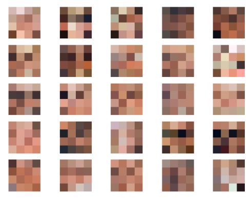
For instance, plot 004x004-tuned.png shows a sample of images created after the first 4×4 training session. We can't see too far at this stage.
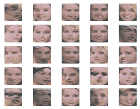
In the same way, these will be the results of 128×128 resolution.

 411+ registered