What is Computational Mechanics?

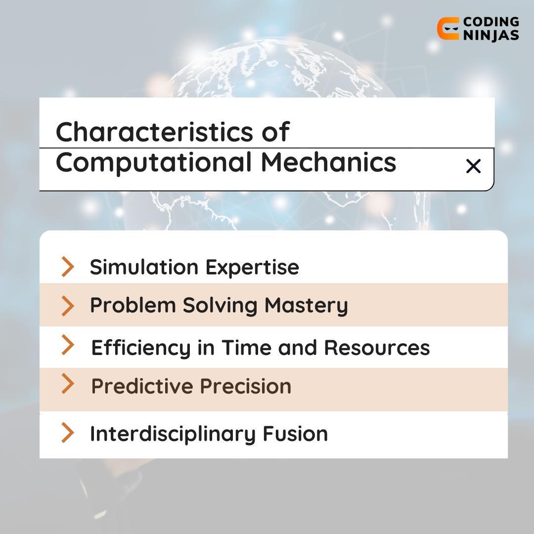
Characteristics of Computational Mechanics

Here are the characteristics of Computational Mechanics that are mentioned below:

Let’s discuss the characteristics of Computational Mechanics.

1. Simulation Expertise

Computational Mechanics is like having a digital laboratory where we create virtual versions of real-world situations. Computational Mechanics relies on computer simulations to replicate real-world actions virtually, providing a digital playground for studying complex phenomena.

2. Problem-Solving Mastery

When things get really complicated, like understanding why bridges stay strong or how water flows, Computational Mechanics steps in. It's like having a secret toolkit of maths and computer tricks. These tools help us break down big problems into smaller pieces that computers can understand. By solving these pieces, we get answers that help us understand the whole puzzle

3. Efficiency in Time and Resources

By digitally testing ideas, Computational Mechanics saves time and resources compared to physical experiments, accelerating innovation. Instead of building actual things to test ideas, imagine if we could try them out on a computer first. This is where Computational Mechanics shines. It saves time because we don't have to wait for real experiments, and it saves money because we don't need all the materials. It's like designing a roller coaster on a computer before building it. If it doesn't work on the computer, we don't waste time and resources building it for real.

4. Predictive Precision

Computational Mechanics uses maths and physics to predict what might happen in different situations. It's a bit like predicting the weather but for things like how bridges will react under heavy loads or how air flows around an aeroplane wing. By simulating these scenarios on computers, we can make sure things are safe and reliable before they're actually built.

5. Interdisciplinary Fusion

Merging insights from mathematics, physics, and computer science, Computational Mechanics crafts accurate simulations for multifaceted real-world challenges.

Think of Computational Mechanics as a meeting point for different subjects. It combines maths, physics, and computer science to create these digital simulations. Imagine a team of experts from different fields working together to solve complex puzzles; that's what happens here. The blend of knowledge from these areas ensures that the simulations are accurate and can handle real-world challenges.

Also see, Mercurial

Advantages of Computational Mechanics

There are various advantages of Computational Mechanics, some of which are listed below:

Let’s discuss about the Advantages of Computational Mechanics

Fast Answers

Computers help us find answers really quickly. It's like having a super-smart friend who can do maths super fast. Instead of waiting a long time to see if things work in real life, we can use computers to try out ideas and see what happens in no time.

Money Saver

With Computational Mechanics, we use virtual tests on computers, so we don't need to spend as much money on materials. Making real things for tests costs a lot of money. But with computers, we can do tests virtually. It's like having a pretend version of something. So, we don't need to spend as much money on materials. This helps save money and resources.

Puzzle Solver

It helps us solve really tough problems by breaking them into smaller parts that computers understand. This way, we can solve big mysteries step by step.

Sometimes problems are really hard to solve, like figuring out how a building can stand strong or how water moves. Computational Mechanics helps by breaking these big problems into smaller, easier parts that computers can understand. It's like solving a puzzle piece by piece.

Safe Exploration

Computers are like a safe playground for testing things. We can try out situations that might be dangerous in real life, but in the computer, there's no real danger. It's like practising without getting hurt. This keeps us safe while learning how things behave under different conditions.

Understanding Complex Stuff

Some things are really complicated, and we can't see them with our eyes alone. Computational Mechanics helps by showing these things with numbers and pictures on the computer. It's like having a special pair of glasses that lets us see hidden details and understand things better.
 

Limitations of Computational Mechanics

The following are the limitations of Computational Mechanics:

Not Always Perfect Predictions

While computers are smart, they can't predict everything perfectly. Sometimes, the real world behaves a bit differently than what the computer says. Computers are like smart helpers, but they don't always get things exactly right. Sometimes, the real world behaves a little differently than what the computer tells us. So, while they're great at guessing, they can't predict everything perfectly.

Complex Learning Curve 

Using Computational Mechanics can be tricky to learn. It's like learning to use a new gadget with lots of buttons and options. Just like learning to use a new toy or gadget with lots of buttons, Computational Mechanics can be challenging to understand. It's like figuring out a new game, it takes time to get really good at it.

Need for Powerful Computers

Solving big problems needs big computer power. Solving big problems needs powerful computers. Not everyone has access to super-powerful computers. Imagine trying to solve a huge puzzle without enough pieces; it's like that. Not everyone has access to these super-powerful computers, which can make things a bit tricky.

Data Dependence

The quality of results depends on good data. If we put in bad data, the computer gives out bad results. It means the computer's answers depend on the information we give it. Just like a robot's cooking skills depend on the ingredients you provide, the computer's accuracy depends on the quality of the data we use. This is why it's really important to double-check and use accurate data so that the computer can give us the best possible answers.

Real-World Proof Required

Imagine you're trying to solve a mystery. Sometimes, you have to check if your guess is right by looking at real clues. Similarly, the computer's guesses need to match with what really happens in the world. We need to test things in real life to make sure the computer's answers are on the right track.

Numerical Techniques of Computational Mechanics

Numerical techniques help us arrange calculations so we can figure out how things behave, making Computational Mechanics a powerful way to understand and solve real-world challenges.

Finite Element Method

The Finite Element Method is a numerical technique employed in Computational Mechanics to analyse and understand complex physical systems. It involves subdividing a larger, intricate problem into smaller, manageable parts called "finite elements." These elements are interconnected at specific points called "nodes." By applying mathematical equations to these elements and nodes, the behaviour and responses of the larger system can be approximated and simulated.

In essence, the method employs mathematical models and computer algorithms to solve complex problems by breaking them down into simpler elements and calculating their interactions. It's a powerful tool used in various fields, including engineering, physics, and materials science, to gain insights into how structures and systems behave under different conditions.

Example

Imagine you're drawing a picture, but instead of drawing the whole thing at once, you draw small parts and put them together to make the whole picture. The Finite Element Method in Computational Mechanics is like that – it's a clever way to understand complex things by breaking them into tiny pieces.

In this method, we pretend that the big thing we're studying is made up of lots of small parts, like a puzzle. Computers use maths to figure out how each small part moves and behaves. By adding up all these small behaviours, we get a clear picture of how the entire thing works.

So, the Finite Element Method is like solving a puzzle one piece at a time using maths and computers. It helps us understand big things by focusing on the small parts and how they fit together.

Mathematical Foundation of the Finite Element Method 
 

Calculus and Linear Algebra

Utilisation of differentiation and integration (calculus) is central for expressing and manipulating equations representing physical behaviours. Linear algebra is pivotal in solving systems of equations resulting from discretization.

Partial Differential Equations 

Governing equations describing the behaviour of physical quantities across space and time, forming the basis for problem formulation.

Variational Calculus and Functional Spaces

Variational calculus aids in deriving weak forms of PDEs, making them amenable to approximation. Functional spaces provide a framework to express the behaviour of functions.

Discretization Concepts

Fundamental understanding of discretization, converting continuous problems into finite elements for analysis.

Shape Functions and Interpolation

Shape functions dictate the variation of quantities within finite elements. Interpolation allows the estimation of values within elements based on nodal values.

Integration Technique

Numerical integration methods, such as Gaussian quadrature, are applied to approximate definite integrals within element equations.

Matrix Algebra and System of Equations

Matrix algebra manipulation plays a key role in handling equations arising from the discretization process.

Boundary Conditions

Skill in incorporating boundary conditions, both essential and natural, ensures meaningful solutions within the mathematical framework.

 

Finite Difference Method

The Finite Difference Method is a numerical technique used to solve partial differential equations or approximate derivatives of a function. It involves discretizing the spatial domain into a grid of points and replacing derivatives with finite difference approximations. By representing continuous derivatives with discrete differences, the method transforms complex differential equations into algebraic equations that can be solved using computers.

In essence, the Finite Difference Method approximates the behaviour of a continuous function by considering the changes in function values at discrete points. It's widely employed in various fields such as physics, engineering, and finance to simulate and analyse diverse phenomena governed by differential equations.

Example

Imagine you're heating a metal rod, and you want to know how the temperature changes along its length over time. The heat conduction equation describes this change, involving both time and space derivatives. The Finite Difference Method lets you discretize time and space into small steps and replaces the derivatives with finite differences.

For the spatial derivative, you choose points along the rod and calculate the difference in temperature between neighbouring points. Similarly, for the time derivative, you calculate how the temperature changes between consecutive time steps.

By substituting these approximations into the heat conduction equation, you get a formula that relates temperatures at different points and times. This equation, with a bit of rearranging, helps you find the temperature at each point and time step.

You then repeat this process, updating temperatures at each point for each time step. 

This gives you a numerical solution that shows how the temperature changes along the rod as time passes.
 

Mathematical Foundation of the Finite Element Method 

The Finite Difference Method is rooted in a discrete approximation of derivatives and integration techniques. Its mathematical foundation involves transforming continuous differential equations into discrete algebraic equations by approximating derivatives using finite differences.

Here's a concise breakdown of the key mathematical components:

Discretization of Space and Time

The method begins by dividing the continuous spatial domain into discrete points along with discretizing time into intervals. This generates a grid where equations will be evaluated.

Taylor Series Expansion

The Taylor series expansion is employed to approximate functions at neighbouring points using derivatives. By truncating the series after a few terms, continuous functions are approximated with discrete differences.

Forward, Backward, and Central Differences

Finite differences are categorised into forward, backwards, and central differences. These approximations quantify how function values change between adjacent grid points and serve as discrete derivatives.

Approximation of Derivatives

In the context of partial differential equations, derivatives are replaced with finite differences in both time and space. These approximations convert continuous equations into discrete forms.

Discretized Equations

By substituting finite difference approximations into the original differential equations, a set of discrete algebraic equations emerges. These equations represent the evolution of the system in a discrete manner.

Stability and Convergence Analysis

The mathematical analysis of stability and convergence ensures that the discrete solution approaches the true solution as grid refinement occurs. Stability conditions are determined to prevent numerical instability.

Implicit and Explicit Methods

The choice between implicit and explicit methods influences the stability and computational efficiency of the solution process. Implicit methods involve solving linear systems at each time step, while explicit methods compute solutions explicitly.

Boundary and Initial Conditions

Just as in continuous problems, boundary and initial conditions are specified in the discrete context. These conditions are incorporated into the discrete equations to capture the problem's behaviour accurately

By approximating derivatives using finite differences, the Finite Difference Method converts complex continuous differential equations into a set of discrete equations that can be solved using numerical techniques. This mathematical foundation underpins its application in solving various scientific and engineering problems.

 

Computational Fluid Dynamics 

Computational Fluid Dynamics is a computational and numerical approach employed to analyse and simulate the behaviour of fluids, such as liquids and gases, by solving complex equations governing fluid motion and behaviour. It involves discretizing the fluid domain into a grid of points, and then employing mathematical equations to approximate fluid flow, heat transfer, and other related phenomena.

CFD operates on the principles of fluid mechanics, thermodynamics, and numerical analysis. By dividing the fluid domain into smaller elements, the governing equations are transformed into discrete algebraic equations that can be solved using computers. This enables predictions and insights into fluid behaviour, including flow patterns, pressure distributions, and temperature changes.

In essence, CFD serves as a virtual laboratory where engineers and researchers can explore and predict how fluids interact with boundaries and other forces under various conditions. Its applications span diverse fields, from aerospace and automotive engineering to environmental modelling, providing insights that aid in design optimization, performance evaluation, and problem-solving within fluid-related systems.

Example

Imagine you're an engineer designing a new car. You want to make sure the car's shape is aerodynamic, meaning it moves smoothly through the air to reduce drag and improve fuel efficiency. This is where Computational Fluid Dynamics (CFD) comes into play.

With CFD, you can create a virtual wind tunnel on your computer. You start by building a 3D model of the car and the surrounding air. Then, you use mathematical equations that describe how air flows around objects to simulate how the air interacts with your car's shape.

Let's say you're particularly interested in how the air flows over the car's body and around its mirrors. CFD allows you to visualise the airflow patterns, identify areas of high pressure (where drag occurs) and areas of low pressure (where lift might happen).

By running simulations with different designs, you can optimise the car's shape to minimise drag and maximise efficiency. You might adjust the curvature of the body, modify the angles of the mirrors, and fine-tune other details based on the insights gained from the CFD simulations.

Ultimately, CFD helps you predict how air will behave around your car without building physical prototypes or conducting expensive wind tunnel tests. It's like having a virtual wind tunnel that guides you to design a sleek and efficient vehicle shape, contributing to better fuel economy and improved performance.
 

Mathematical Foundation of the Finite Element Method 

The Mathematical Foundation of Computational Fluid Dynamics (CFD) is built upon principles from fluid mechanics, numerical analysis, and computational methods. It involves transforming the fundamental equations governing fluid flow into discrete forms suitable for numerical approximation on computers. 

Here's a concise exploration of its key mathematical components:

Navier-Stokes Equations

The Navier-Stokes equations describe the motion of fluid and are the cornerstone of fluid dynamics. These equations capture the conservation of mass, momentum, and energy, providing a mathematical representation of fluid behaviour.

Discretization of Space and Time

To solve complex fluid equations numerically, the continuous spatial domain is discretized into a grid of cells or elements. Similarly, time is divided into discrete intervals.

Finite Volume or Finite Difference Methods

Numerical methods like finite volume or finite difference techniques approximate derivatives by analysing changes in values between neighbouring grid points. These methods transform differential equations into algebraic equations on a grid.

Conservation Principles

CFD relies on the conservation laws of mass, momentum, and energy. Numerical schemes must uphold these principles to ensure accurate simulation results.

Boundary Conditions

As in physical fluid systems, CFD requires the specification of boundary conditions to accurately represent the fluid's interaction with its surroundings. These conditions constrain the solutions and often involve enforcing prescribed values or gradients at boundaries.

Time Stepping Schemes

Temporal advancement of simulations involves time-stepping schemes that dictate how values evolve from one time level to the next. Implicit and explicit methods balance stability and computational cost.

Turbulence Modelling

For turbulent flows, turbulence models are incorporated to approximate the intricate behaviour of eddies and fluctuations. These models introduce additional equations to account for turbulent effects.

Solution Algorithms

Systems of algebraic equations arising from discretized equations are solved iteratively using linear solvers or advanced methods like multigrid techniques.

Visualisation and Interpretation

Results from CFD simulations provide insight into fluid behaviour through visual representations of velocity vectors, pressure contours, and other flow characteristics.

Boundary Element Method 

The Boundary Element Method is a numerical technique used to solve engineering and mathematical problems involving partial differential equations (PDEs) by focusing on the boundaries of the domain. Unlike traditional numerical methods that discretize the entire domain, BEM strategically discretizes only the boundary, exploiting the fact that many physical problems can be accurately described by their boundary behaviour.

In BEM, the boundary of the problem domain is divided into elements, and the solution is sought directly on this boundary. The method formulates integral equations based on the fundamental solution of the governing PDE, often exploiting Green's function concept. By solving these integral equations, BEM provides a powerful approach to solving problems in potential theory, fluid dynamics, heat conduction, and elasticity, among others.

Boundary Element Method is particularly advantageous for problems with infinite or unbounded domains, as it requires discretization only on the boundary. This approach reduces the computational effort compared to volumetric discretization methods like the Finite Element Method. It's also well-suited for problems with singularities or concentrated forces since it naturally captures boundary effects.

Example 

Imagine you're an engineer working on designing a dam to control water flow in a river. To ensure the dam's stability, you need to analyse how water pressure interacts with the dam structure. This is where the Boundary Element Method (BEM) can be applied effectively.

Using the Boundary Element Method, you discretize the surface of the dam into small elements, like triangles or rectangles. These elements define the dam's boundary, which is crucial for understanding how water pressure affects it. Instead of dividing the entire space around the dam, you focus on its surfaces.

The next step is to formulate integral equations based on the fundamental solution of the Laplace equation. This solution characterises the distribution of fluid pressure around the dam. By solving these equations on the dam's boundary, you can determine how water pressure varies across its surface.

BEM's advantage is that you avoid the need to create a mesh for the entire volume of water. Instead, you concentrate on the dam's surfaces, where the interaction with water occurs most significantly.

By solving the integral equations, you can visualise the pressure distribution on the dam's surface. This insight is crucial for ensuring that the dam structure can withstand the forces exerted by the water pressure, contributing to a safe and stable design.

 

Mathematical Foundation of the Finite Element Method 

The Boundary Element Method (BEM) is grounded in mathematical principles that focus on discretizing the boundary of a problem domain to solve partial differential equations (PDEs). 

This method transforms the PDEs into integral equations, allowing the solution to be determined directly on the boundary. 

Here's a concise overview of its key mathematical elements:

Fundamental Solution and Integral Equations 

BEM relies on the concept of the fundamental solution, a mathematical function that satisfies the governing PDE. Integral equations are formulated based on this fundamental solution, relating values of the unknown field on the boundary to known values and derivatives.

Boundary Discretization

The boundary of the problem domain is divided into smaller elements, often triangles or quadrilaterals in two dimensions and triangles or tetrahedra into three dimensions. These elements define the discrete approximation of the boundary.

Galerkin or Collocation Method

Integral equations are solved using either the Galerkin method, which involves choosing specific trial functions to minimise the residual error, or the collocation method, where integral equations are evaluated at discrete collocation points.

Singular and Hypersingular Integrals

BEM equations often involve integrals with singular or hypersingular kernels due to their proximity to the integration points. Techniques like regularisation or special numerical integration rules address these challenges.

Green's Function

The fundamental solution is often represented as a Green's function. This function encapsulates the influence of a point source on the field of interest, allowing integral equations to be formulated and solved.

Linear System Solvers

The integral equations lead to a linear system of equations. Techniques like Gaussian elimination, LU decomposition, or iterative solvers are used to solve this system and determine the unknown values on the boundary.

Domain Mapping (2D to 3D)

In three-dimensional problems, BEM often employs domain mapping techniques to transform the problem into two dimensions, simplifying the boundary discretization and integral equation formulation.

Boundary Conditions

Essential and natural boundary conditions are incorporated into the integral equations to enforce constraints and accurately model the problem's behaviour.

Challenges of Computational Mechanics 

There are various challenges of Computational Mechanics, some of which are listed below:

These challenges show that Computational Mechanics needs careful handling to accurately simulate and understand complex real-world behaviours.

1. Tricky Problems: Solving complex issues requires detailed models, which can take a lot of time and computer power.

2. Getting it Right: Striking a balance between accurate results and quick calculations is tough. More detail often means slower simulations.

3. Grid Trouble: Creating the right grid for simulations is a challenge. Small mistakes in grid design can affect results.

4. Realistic Behaviour: Some problems, like materials bending or breaking, are hard to describe exactly in simulations.

5. Checking Reality: Trusting simulation results means comparing them to real-world data, but this isn't always possible.

Applications of Computational Mechanics 

Computational Mechanics is super useful in many areas:

1. Building Safety: It checks how structures can handle earthquakes or strong winds, keeping us safe in buildings.

2. Air and Space Travel: It figures out how aeroplanes and rockets can fly smoothly, making our journeys safer.

3. Car Crash Testing: It helps design cars that protect us during accidents by simulating crashes.

4. Weather Forecast: Scientists use it to predict weather patterns, helping us prepare for storms.

5. Medical Implant: It ensures that devices like artificial hips work well inside our bodies.

6. Energy Efficiency: It makes power plants and green energy sources better at producing electricity.

7. Product Making: It helps create better products, from phones to cars, by understanding how materials behave.

8. Environmental Impact: It studies how big projects affect nature, helping us make smarter decisions.

9. Stronger Materials: Scientists develop new materials, like tough metals, using these simulations.

10. Fluid Behaviour: It looks at how fluids move, like water in pipes or blood in our bodies.
 

Frequently Asked Questions

How does Computational Mechanics work?

Computational Mechanics breaks down real-world problems into smaller mathematical elements, which are then solved using computer algorithms. The solutions provide insights into how systems behave under different conditions.

How accurate are the results from Computational Mechanics simulations?

The accuracy of Computational Mechanics simulations depends on various factors. Well-validated models and accurate input data can lead to reliable predictions. However, there are trade-offs between accuracy and computational speed. Ensuring that simulations are validated against real-world data helps improve their reliability and build confidence in the results. It's important to understand that simulations provide valuable insights but should always be accompanied by critical analysis and validation.

What is the future of Computational Mechanics?

The future involves integrating artificial intelligence with simulations, making simulations more accessible through cloud computing, and handling increasingly complex multi-physics problems.

Conclusion

Computational Mechanics is a dynamic field that uses computer simulations to tackle complex real-world challenges. By breaking down intricate problems into manageable digital models, it empowers engineers, scientists, and researchers to design safer structures, predict natural phenomena, optimise technologies, and explore new frontiers. As technology advances, Computational Mechanics continues to play a pivotal role in shaping innovations across various disciplines, making our world safer, more efficient, and better understood.

Refer to our Guided Path to upskill yourself in DSA, Competitive Programming, JavaScript, System Design, and many more! If you want to test your competency in coding, you may check out the mock test series and participate in the contests hosted on Coding Ninjas Studio!

But suppose you have just started your learning process and are looking for questions from tech giants like Amazon, Microsoft, Uber, etc. For placement preparations, you must look at the problems, interview experiences, and interview bundles.

We wish you Good Luck! 

Happy Learning!