Do you think IIT Guwahati certified course can help you in your career?
Introduction
Topic modelling is extracting the central subjects from a body of text using a quantitative method. It's like PCA, which finds the important quantitative patterns (that explain the greatest variance) in your features. PCA's outputs are a technique of condensing our features – for example, it can reduce a list of 500 features to 10 summary features. These ten features are essential topics.
We are going to learn how to do topic modelling with the help of a statistical technique, Nonnegative Matrix Factorization.
Nonnegative Matrix Factorization (NMF)
Matrix with Nonnegative Values Factorization is a statistical strategy for reducing the dimension of an input corpus or corpus. Internally, it employs the factor analysis method to assign a lower weighting to less coherent words.
1. It is a member of the linear algebra algorithm family that is used to find the latent or hidden structure in data.
2. It takes the form of a nonnegative matrix.
3. It can also be used for topic modelling, with the term-document matrix as the input, which is usually TF-IDF normalized.
Input: Number of subjects, Term-Document matrix
Output: Two nonnegative matrices of the original n-words by k topics and the same k topics by m original documents are returned.
To put it another way, we use linear algebra to model topics.
4. NMF's popularity stems from its ability to automatically extract sparse and easily interpretable factors.
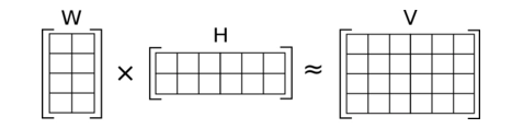
The following is a diagram of the technique described above:
As shown in the diagram above, we start with the term-document matrix (A), which we deconstruct into two matrices.
The first matrix contains every topic and all of the associated terms; the second matrix contains every document and all of the topics associated with it.
General case of NMF:
Let's consider a general situation of NMF, where the input matrix V has the shape m x n. This topic modelling method divides the matrix V into two matrices, W and H, with W and H having the shapes m x k and k x n, respectively.
The following is how different matrices are interpreted in this method:
The V matrix represents the term-document matrix.
Each row of matrix H represents a word embedding.
W matrix: Each column of the W matrix indicates the weightage that each word receives in each sentence or the semantic relationship between words and sentences.
However, the most critical assumption is that all matrices W and H's elements are positive if all of V's entries are positive.
Maths behind NMF
NMF, as previously stated, is a type of unsupervised machine learning technique. Unsupervised learning's primary purpose is to quantify the distance between the parts. We have numerous ways of measuring distance however in this blog article, we will focus on two popular methods used by Machine Learning practitioners: - Generalized Kullback–Leibler divergence - Frobenius norm
Let's discuss each of them one by one in a detailed manner:
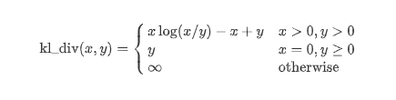
Generalized Kullback–Leibler Divergence
It's a statistical measure that determines how distinct one distribution is from another. As the Kullback–Leibler divergence approaches 0, the similarity of the similar words grows, or in other words, the divergence value decreases.
The formula for calculating the is as follows:
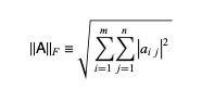
Frobenius Norm
It's a different way of doing NMF. The sum of absolute squares of its square root constituents defines it. The euclidean norm is another name for it. The Frobenius Norm is calculated using the following formula:
Objective Function in NMF
We must obtain two matrices, W and H, from the initial matrix A, such that
WH= A
W and H described the following information about matrix A using NMF's intrinsic clustering property:
A (Document-word matrix) is information that shows which words appear in which documents.
The subjects (clusters) discovered from the documents are referred to as W (Basis vectors).
The membership weights for the themes in each document are represented by H (coefficient matrix).
We can state that we have an optimization procedure to develop the model and seek to reach high accuracy based on our prior understanding of Machine and Deep learning. With the scikit-learn package, there are two types of optimization methods.
Coordinate Descent Solver
Multiplicative update Solver
In this technique, we can calculate matrices W and H by optimizing over an objective function (like the EM algorithm), and update the matrices W and H iteratively until convergence.
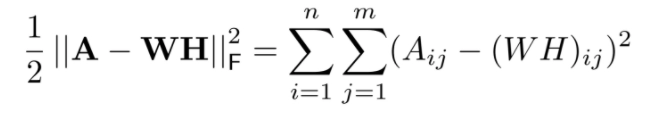
This is the objective function of NMF.
On the basis of Euclidean distance, we aim to estimate the reconstruction error between matrix A and the product of its elements W and H in this objective function.
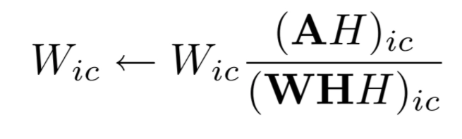
Our update rules for W and H can now be derived using the objective function, and we get:
Matrix W elements should be updated as follows:
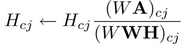
Matrix H elements should be updated as follows:
We update the values in parallel and then compute the reconstruction error using the new matrices we acquire after updating W and H. We repeat this approach until we reach convergence.
As the last step, we can claim that this technique will change the initial values of W and H up to the product of these matrices' approaches to A, or until the approximation error converges or the maximum number of iterations is reached.
The high-dimensional vectors or initialized weights in the matrices will be TF-IDF weights in our case, but anything can be used, including word vectors or a simple raw count of the words. However, various strategies for initializing these matrices to get rapid convergence or a satisfactory solution. Let's talk about those heuristics in the next part.
We can initialize the matrices randomly.
Real-life Application of NMF
Image Processing uses the NMF. Let's look at more details about this.
Let's say we have a p-pixel grey-scale image of a face, and we want to compress the data into a single vector, with the ith entry representing the value of the ith pixel. Let the p pixels be represented by the rows of X R(p x n), and the n columns are one image each.
Now, we'll use the NMF to create two matrices, W and H, in this application. A question may now arise in your mind:
What do these matrices indicate in relation to the Use-Case in question?
Matrix W: W's columns can be thought of as pictures or basic images.
Matrix H: This matrix instructs us on how to sum the basis photos in order to reconstruct a face approximation.
The following features can be used as the primary images for facial images:
Eyes,
Noses,
Moustaches,
Lips
The H columns indicate which features are present in each image.
Frequently Asked Questions
1. Is nonnegative matrix factorization unsupervised? In its classical form, NMF is an unsupervised method, i.e. the class labels of the training data are not used when computing the NMF. 2. What is nonnegative matrix factorization used for? Nonnegative matrix factorization (NMF) has become a widely used tool for the analysis of high dimensional data as it automatically extracts sparse and meaningful features from a set of nonnegative data vectors. 3. How do you factor a nonnegative matrix? Approximate nonnegative matrix factorization, Usually, the number of columns of W and the number of rows of H in NMF are selected so the product WH will become an approximation to V. The complete decomposition of V then amounts to the two nonnegative matrices W and H as well as a residual U, such that: V = WH + U 4. Which is better, LDA or NMF? The observed results show that both the algorithms perform well in detecting topics from text streams, the results of LDA being more semantically interpretable while NMF is faster of the two.
Conclusion
So, in a nutshell, Non-Negative Matrix Factorisation is a powerful technique for analysing high dimensional data and taking meaningful features out of it.
Hey Ninjas! Don't stop here; check out Coding Ninjas for Machine Learning, more unique courses, and guided paths. Also, try Coding Ninjas Studio for more exciting articles, interview experiences, and fantastic Data Structures and Algorithms problems.


 6+ registered

