


Introduction
The Gibbs Sampling is a Monte Carlo Markov Chain strategy that iteratively draws an occasion from the conveyance of every variable, contingent on the current upsides of different factors to assess complex joint dispersions. Gibbs is utilized in LDA as it forestalls relationships between's examples during the emphasis. We will use the LDA work from the topic models library to execute Gibbs inspecting strategy on a similar arrangement of crude records and print out the outcome for us to look at.
Gibbs Sampling in LDA
Text clustering is a generally utilized strategy to draw out designs from many archives naturally. This idea can be reached to the client division in the advanced advertising field. One of its fundamental centers is to get what drives guests to come, leave and act nearby. One straightforward method for doing this is auditing words that they used to show up on location and what words they utilized ( what things they looked ) when they're on your site.
One more utilization of text clustering is for archive association or ordering (labeling). With plenty of data accessible on the Internet, the executives' subject of the information has become more significant. What's more, that is the place where labeling comes in. Everybody's perspective about things might contrast somewhat; a group of data designers might contend over which word is the correct term to address a record for quite a long time. An LDA Gibbs Sampling calculation - can be inferred for all of these inactive factors; we note that both θd and φ(z) can be determined utilizing only the subject record tasks.
Gibbs sampling
Gibbs sampling is named after the physicist Josiah Willard Gibbs, regarding a relationship between the sampling calculation and measurable material science. The analysis was depicted by siblings Stuart and Donald Geman in 1984, about eighty years after the passing of Gibbs.
Gibbs sampling is an extraordinary instance of the Metropolis-Hastings calculation in its basic form. Nonetheless, in its lengthy variants (see beneath), it tends to be viewed as an overall structure for sampling from an enormous arrangement of factors by sampling every variable (or, at times, each gathering of elements) like this. It can join the Metropolis-Hastings calculation (or techniques, for example, cut sampling) to execute at least one of the sampling steps.
Gibbs sampling is material when the joint dispersion is not known expressly or is challenging to test straightforwardly. However, the contingent dissemination of every variable is known and is simple (or possibly, more straightforward) to test from. The Gibbs sampling calculation creates an example by disseminating every variable, contingent on the current upsides of different factors. It tends to be shown that the grouping of tests comprises a Markov chain, and the fixed circulation of that Markov chain is only the pursued joint dissemination.
Gibbs sampling is especially all-around adjusted to sampling the back dissemination of a Bayesian organization since Bayesian organizations are commonly indicated as
an assortment of restrictive circulations.
If we take a gander at this in a numerical way, what we are doing is we are attempting to observe restrictive probability appropriation of a solitary word's theme task adapted to the remainder of the point tasks. Overlooking every one of the numerical computations, what we will get is a contingent probability condition that resembles this for a solitary word w in record d that has a place with subject k:
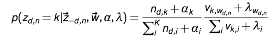
where:
n(d,k): Number of times report d use point k
v(k,w): Number of times theme k purposes the given word
αk: Dirichlet boundary for the information to point appropriation
λw: Dirichlet boundary for the subject to word circulation
There are two sections two this condition. The initial segment lets us know how much every theme is available in a report, and the next part tells how much every point loves a word. Note that we will get a vector of probabilities for each word that will make sense of how likely this word has a place with every one of the subjects. In the above condition, it very well may be seen that the Dirichlet boundaries additionally go about as smoothing edges when n(d,k) or v(k,w) is zero, which intends that there will, in any case, be some opportunity that the word will pick a point going ahead.
Latent Dirichlet Allocation (LDA)
Latent Dirichlet Allocation (LDA) is a probabilistic theme demonstrating a technique that gives us a way to deal with coaxing out potential subjects from archives that we do not know about in advance. The strong presumption behind LDA is that each given archive is a blend of numerous points. Given many records, one can utilize the LDA structure to learn not just the subject blend (dispersion) that addresses each report. However, in addition, words (circulation) related to every point to assist with understanding what the theme may allude to.
The theme dispersion for each record is disseminated as
θ∼Dirichlet(α)
Where Dirichlet(α) signifies the Dirichlet dissemination for boundary α.
The term (word) conveyance, then again, is likewise demonstrated by a Dirichlet dissemination, simply under an alternate boundary η ( articulated "estimated time of arrival," you will see different spots allude to it as β ).
ϕ∼Dirichlet(η)
The most significant possible level of the objective of LDA is to gauge the θ and ϕ, which is comparable to appraising which words are significant for which theme and which subjects are significant for a specific report separately.
The fundamental thought behind the boundaries for the Dirichlet appropriation ( here I am alluding to the even form of the circulation, which is the overall case for most LDA) is: α The higher the worth, the almost certain each archive is to contain a combination of a large portion of the points rather than any single theme. The equivalent goes for η, where higher worth means that every point will probably contain a combination of the more significant part of the words and no word explicitly.
There are various ways to deal with this calculation, the one we will utilize is Gibbs sampling. We will utilize 8 short strings to address our arrangement of records. The accompanying segment sets the reports and converts each record into word ids, where word ids is only the ids relegated to every remarkable word in the archive arrangement. We're dropping the issue of stemming words, eliminating various blank areas, and other normal preprocessing steps while performing text mining calculations as this is a genuinely straightforward arrangement of reports.
- Θtd = P(t|d) which is the probability conveyance of subjects in archives
- Фwt = P(w|t) which is the probability appropriation of words in points
What's more, we can say that the probability of a word given record for example P(w|d) is equivalent to:
tT=p(w|t,d) p(t|d)
where T is the absolute number of subjects. Additionally, we should accept that there is W number of words in our jargon for every one of the records.
On the off chance that we accept contingent freedom, we can say that
P(w|t,d) = P(w|t)
What's more, henceforth P(w|d) is equivalent to:
t=1T=p(w|t) p(t|d)
that is the speck result of Θtd and Фwt for every subject t.
This can be addressed as a network like this:
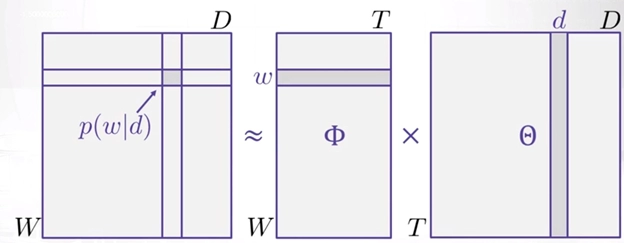
Along these lines, taking a gander at this we can imagine LDA like that of framework factorization or SVD, where we decay the probability appropriation network of words in the record in two lattices comprising of dispersion of point in an archive and conveyance of words in a theme.
Example with code
Let's take the following data
W = np.array([0, 1, 2, 3, 4])


# D := document words
X = np.array([
    [0, 0, 1, 2, 2],
    [0, 0, 1, 1, 1],
    [0, 1, 2, 2, 2],
    [4, 4, 4, 4, 4],
    [3, 3, 4, 4, 4],
    [3, 4, 4, 4, 4]
])


N_D = X.shape[0]  # num of docs
N_W = W.shape[0]  # num of words
N_K = 2  # num of topics
This information is now in a pack of words portrayal, so it is somewhat conceptual initially. Anyway, on the off chance that we take a gander at it, we could see two major bunches of records given their words: {1,2,3} what's more, {4,5,6}. Along these lines, we expect that the point dissemination for those archives will follow our instinct after our sampler joins to the back after our sampler joins.
Output
Document topic distribution:
----------------------------
[[ 0.81960751  0.18039249]
 [ 0.8458758   0.1541242 ]
 [ 0.78974177  0.21025823]
 [ 0.20697807  0.79302193]
 [ 0.05665149  0.94334851]
 [ 0.15477016  0.84522984]]
As may be obvious, to be specific, documents 1, 2, and 3 will quite often be in a similar group. The equivalent could be said for documents 4, 5, and 6.

 6+ registered

