Feature Scaling

Normalization v/s Standardization v/s Robust Scaling

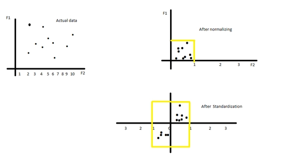
The debate about normalization vs. standardization vs. robust scaling is a perennial one among machine learning newbies. In this section, I'll expand on the response.

Normalization	Standardization	Robust Learning
When you know that your data does not follow a Gaussian distribution, normalization is a suitable option. Normalization is helpful in algorithms like K-Nearest Neighbors and Neural Networks, which do not presume any data distribution.   The range of Normalization is from 0 to 1. As a result, even if your data contains outliers, normalization will not affect them.	In circumstances where the data follows a Gaussian distribution, on the other hand, standardization can be beneficial. However, this is not the case all the time.    Standardization, unlike normalization, does not have a bounding range.  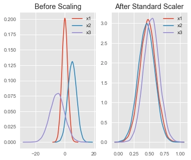Standardization subtracts the mean, and then it divides by the standard deviation to ensure that the mean is equal to 0 and the scales become comparable in terms of standard deviation. In the case of outliers, this leads to overperformance.	If your dataset has many outliers, one or both of the most important procedures – Standardization and Normalization – may not perform as well. This problem can be solved with robust scaling.    We can solve the problem of outliers by scaling the dataset suitably with the RobustScaler in Scikit-learn, limiting the range but maintaining the outliers to continue to contribute to feature importance and model performance.

 

Source

However, whether you use normalization, standardization, or robust learning depends on your problem and the machine learning algorithm you're utilizing at the end of the day. When it comes to normalizing or standardizing your data, there is no hard and fast rule. To get the best results, start by fitting your model to raw, normalized, and standardized data and comparing the results. And if you have a lot of outliers in your dataset, then try using robust learning.

Types of Feature Scaling techniques and how to do it

To demonstrate different feature scaling strategies, we'll use the SciKit-Learn library. You can download the Salary CSV file from here. Let's start coding! We are going to look at the data first before scaling it.

#imports
import numpy as np
import pandas as pd
import matplotlib.pyplot as plt
import seaborn as sns
#reading the csv file and making it into dataframe
data = pd.read_csv("../Downloads/Salary_Data.csv")
#function to plot graph after feature scaling 
def make_scatter_plot(data):
    x=data["YearsExperience"].to_numpy()
    y=data["Salary"].to_numpy()
    plt.xlabel("Years of Experience")
    plt.ylabel("Salary")
    plt.scatter(x,y)
    print(plt.show())
print("Data before Scaling")
data.head(5)

 

 

make_scatter_plot(data)#calling function to make graph

 

Standard Scaler/ Standardization

In this method, we center the feature at 0 with a standard deviation of 1. Hence, bringing all of the parameters to a similar scale. This technique will be affected if there are any outliers. As a result, we use this with only normally distributed features.

 

Source

 

This method of rescaling features with a distribution value between 0 and 1 is beneficial for optimization methods like gradient descent, used in machine learning techniques to weight inputs (e.g., regression and neural networks). For algorithms that require distance measurements, such as K-Nearest-Neighbours, rescaling is also used (KNN).

 

 

Source

 

from sklearn.preprocessing import StandardScaler #import
standard_scaler=StandardScaler()
standard_scaled_data=pd.DataFrame(standard_scaler.fit_transform(data),columns=data.columns)
print("Data after Standard Scaling")
standard_scaled_data.head(5)

 

make_scatter_plot(standard_scaled_data)#calling function to make graph

 

Min-Max Scaler/ Normalization 

This estimator scales each feature separately to fall inside the specified range, between zero to one. This method is primarily utilized in deep learning, although it can also be employed when the distribution is not Gaussian. Outliers are also taken into account by this scaler.

This type of scaling strategy is applied when the data has a wide range of applications and the algorithms used to train the data, such as Artificial Neural Networks, do not make assumptions about the data distribution.

 

Source

 

Where,

x= any value in the feature column

x min= Minimum value in the feature column

x max= Maximum value in the feature column

x scaled= x after being scaled

 

from sklearn.preprocessing import MinMaxScaler #imports
minmax_scaler=MinMaxScaler()
minmax_scaled_data=pd.DataFrame(minmax_scaler.fit_transform(data),columns=data.columns)
print("Data after MinMax Scaling")
minmax_scaled_data.head(5)

 

make_scatter_plot(minmax_scaled_data)#calling function to make graph

 

Robust Scaler

When we have outliers in our data, this is a very reliable technique. This technique removes the median and scales the data according to the quartile range. Scaling with the mean and standard deviation will not work if our data contains many outliers. As a result, it scales the data using the interquartile range.

Calculate the median (50th percentile), as well as the 25th and 75th percentiles. After subtracting the median from each variable's value, the interquartile range (IQR), the gap between the 75th and 25th percentiles, is divided.

 

value = (value – median) / (p75 – p25)

Where,

p25, p75 = 25th and 75th percentiles

 

from sklearn.preprocessing import RobustScaler
robust_scaler=RobustScaler()
robust_scaled_data=pd.DataFrame(robust_scaler.fit_transform(data),columns=data.columns)
print("Data after Robust Scaling")
robust_scaled_data.head(5)

 

make_scatter_plot(robust_scaled_data)#calling function to make graph

 

Gaussian Transformation

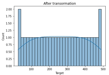
If our features are not normally distributed, and we have skewed data, we can use transformations to make them distributed. I am showing the techniques through the code itself because it is pretty much self-explanatory.

import scipy.stats as stat #import for boxcox tranformation
import pylab

 

We can use the techniques given below:

Logarithmic Transformation

Source

Source

Where,

y= Dependent feature

x= Independent feature

 

In the image above, we see that logarithmic transformation helps us find the best fit line by distributing the features normally.

data_logarithmic=data.copy()
data_logarithmic["Salary_log"]=np.log(data["Salary"])

 

Reciprocal Transformation

x=np.arange(5,100,3) #feature
y=1/x+5 #target
rec_y=x+5 #reciprocal transformation of the target
#target vs feature
plt.xlabel("Feature")
plt.ylabel("target")
plt.title("Target v/s feature")
sns.regplot(x=x,y=y,data=None)
# 1/Target vs feature
plt.xlabel("Feature")
plt.ylabel("1/ Target")
plt.title("1/Target vs feature")
plt.scatter(x,rec_y)
plt.plot(x,rec_y)
plt.show()

 

#data distribution before transformation
plt.title("Before transformation")
plt.xlabel("Target")
sns.histplot(y,kde=True,bins=30)
#data distribution after tranformation
plt.title("After transformation")
plt.xlabel("Target")
sns.histplot(rec_y,kde=True,bins=30)

 

data_reciprocal=data.copy()
data_reciprocal["Salary_rec"]=1/data["Salary"]

 

Square Root transformation

x2=np.arange(5,200,7)#feature
y2=(x2+5)**(2)#target
sqroot_y=x2+5 #square root transformation of the target
#target vs feature
plt.xlabel("Feature")
plt.ylabel("target")
plt.title("Target v/s feature")
sns.regplot(x=x2,y=y2,data=None)
#target^½ vs feature
plt.xlabel("Feature")
plt.ylabel("Target^1/2")
plt.title("Target^1/2 vs feature")
plt.scatter(x2,sqroot_y)
plt.plot(x2,sqroot_y)
plt.show()

 

#data distribution before transformation
plt.title("Before transformation")
plt.xlabel("Target")
sns.histplot(y2,kde=True,bins=30)
#data distribution after tranformation
plt.title("After transformation")
plt.xlabel("Target")
sns.histplot(sqroot_y,kde=True,bins=30)

 

 

data_sqroot=data.copy()
data_sqroot["Salary_sqroot"]=data["Salary"]**(1/2)

 

Exponential Transformation

x3=np.arange(5,100,3)#feature
y3=(x3*5)**(1.2)#target
expo_y=x3*5 #exponential transformation of the target
#Target vs feature
plt.xlabel("Feature")
plt.ylabel("target")
plt.title("Target v/s feature")
sns.regplot(x=x3,y=y3,data=None)
#Target^(1/1.2) vs feature
plt.xlabel("Feature")
plt.ylabel("Target^(1/1.2)")
plt.title("Target^(1/1.2) vs feature")
plt.scatter(x3,expo_y)
plt.plot(x3,expo_y)
plt.show()

 

#data distribution before transformation
plt.title("Before transformation")
plt.xlabel("Target")
sns.histplot(y3,kde=True,bins=30)
#data distribution after tranformation
plt.title("After transformation")
plt.xlabel("Target")
sns.histplot(expo_y,kde=True,bins=30)

 

data_exponential=data.copy()
data_exponential["Salary_exp"]=data["Salary"]**(1/1.2)

 

Box-Cox Transformation

Source

data_boxcox=data.copy()
data_boxcox["Salary_box"],parameters= stat.boxcox(data["Salary"])

Frequently Asked Questions

1. Do all machine learning algorithms require feature scaling?
   Ans. Some algorithms, such as Decision Trees and Ensemble Techniques (including AdaBoost and XGBoost), do not require scaling because their splitting is based on values.
    
2. At which step in the code should we do scaling?
   Ans. It is essential to perform scaling after splitting the data into training and testing. If we don't do this, there will be data leakage from test data to train data.
    
3. What is the best scaling technique and why?
   Ans. There is nothing like the most effective transformation/scaling procedure. It all relies on the type of data you have and how well you know your business. In some cases, some scaling techniques improve the accuracy and performance of the algorithms, while other techniques improve accuracy and performance in different models.

Key Takeaways

In this article, we looked at what Feature Scaling is and how to do it in Python with Scikit-Learn using StandardScaler for standardization and MinMaxScaler for normalization.

The technique of scaling the values of features to a more manageable size is usually done during the preprocessing step. If you want to know about more applications of Feature Scaling, then check out our industry-oriented machine learning course curated by our faculty from Stanford University and Industry experts. 

Recommended Readings:

• GCD Euclidean Algorithm