Lexical Scoping in R

Why is Lexical Scoping?

A lexical scoping is the set of rules that are imposed on the program's variables and functions. It is also known as static scoping. Via lexical scoping, a function is able to access variables from the parent to the global scope. Thus a child function is lexically bound to the parent function. While using lexical scoping, we only need to look at the function definition and not the function nesting to know the value of a variable.

The term lexical in lexical scoping is not the same as the usual English definition. In computer science, lexing is a process that converts code into meaningful pieces which are clear to understand by a programming language.

Principles of Lexical Scoping

R uses four basic principles in order to implement lexical scoping, which are as follows.

1. Name Masking
2. A fresh start
3. Functions vs. variables
4. Dynamic Lookup
    

Let us now discuss each one of them in detail.

Name Masking

This principle states that a name defined inside a function masks the names outside the function. Let's try to understand this statement through various scenarios.

When a variable is not defined in the function:

Let us now look at the case where a variable is not declared and defined in the function.

Code

x <- 10
sum <- function(y, z) {
    x + y + z 
}
# Calling the sum function
sum(20, 30)

Output

Explanation

In the above example, the variable x is not defined in the sum() function. Thus, R looks one level above and assigns values 10 to variable x. After computing the results, it is returned to the caller function.
 

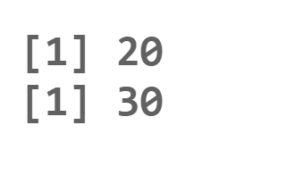
When the name is not defined in the function:

The same rule as the previous case can be applied to this case as well.

Code

x <- 10
y <- 30
add <- function() {
    y <- 10
    x + y 
}
# Calling the add function
add()
# Printing the y variable
y

Output

Explanation

In the above example, the name of variable x is not defined in the add() function. R looks for this variable one level above, and the result is returned to the caller function. We can notice the value of variable y remains unchanged outside the scope of function.
 

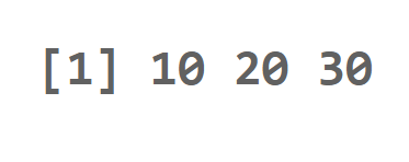
When a function is defined inside another function:

The same rule is applied when a function is defined in some other function. Let us look at an example of the same.

Code

x <- 10
fun1 <- function() {
    y <- 20
    fun2 <- function(){
        z <- 30
        fun3 <- function(){
            c(x, y , z)
        }
        # Calling fun3
        fun3()
    }
    # Calling fun2
    fun2()
}
# Calling fun1
fun1()

Output

Explanation

In the above example, we have a nesting of functions from fun1 to fun3. When fun3 is executing, it looks for all variables one level above the global scope until it finds all values of variables. After getting the variable values, we used the c() function to combine those variables.
 

When functions are created by some other functions:

In R, closures are used to create functions within a function. The same rules of lexical scoping are applied to the closures in R.

Code

add <- function(a){
    b <- 20
    function(){
        # adding both variables
        a + b
    }
}
compute <- add(10)
# Calling compute function
compute()

Output

Explanation

In the above example, we can observe that the function compute() preserves the values of variables a and b in its environment. After performing calculations, the compute() function prints our output.

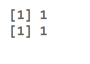
A Fresh Start

A fresh start refers to the concept that each time a function is invoked, a new environment is created. This environment is independent of previous invocations of the same function. Using this concept, R ensures a new and fresh environment creation for each function call.

Let us now look at what happens to the values of variables between invocations of functions. Let's create a function and call it multiple times to analyze the value of variables.

Code

check <- function() {
    if (!exists("a")) {
        a <- 1
    } else {
        a <- 0
    }
    a
}
# First call
check()
# Second call
check()

Output

Explanation

In the above example, we can see that each time we call the check function, it returns the same result. This happens because in R, every time a function is called, a new environment is created for its execution. Thus, a function cannot tell what happened the last time it was run. 

Note: If you don’t know about exist() function, it returns a boolean TRUE value; if there is a variable with that value else, it returns FALSE.

Functions vs Variables

In R, functions are also ordinary objects. Thus, all the scoping rules we have applied for variables also apply to functions.

Code

# Global declaration of helper function
helper <- function(x){
    x + 1
} 
compute <- function(){
    helper <- function(x){
        2 * x 
    }
    
    helper(10)
}
# Calling the function
compute()

Output

Explanation

In the above example, we created a compute function, which has a local helper function in its environment. We also have a global declaration of helper function. Now, whenever we call the compute function, the helper function in compute is called, R looks up for the helper function in the same environment and then levels up to the parent environment if not found. As we have the helper function in the same environment, it computes and returns 20.

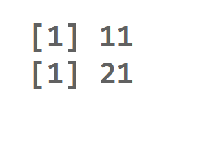
Dynamic Lookup

Lexical scoping tells us where to look for values but not when to look for them. R looks for the values when the function is running but not when it is created. The output of the function can be distinct depending on objects outside its environment.

Code

increment <- function() x + 1
x <- 10
# First call
increment()

x <- 20
# Second call
increment()

Output

This behaviour can be quite bothersome. When we create a function and if we make a spelling mistake in our code, we will not get an error message. To detect this problem, we can use the findGlobals() from the codetools.

Code

increment <- function() x + 1 
x <- 10
# First call
increment()

x <- 20
# Second call
increment()

# Finding global variable of increment
codetools::findGlobals(increment)

Output

Explanation

In the above example, we used the findGlobals() function to detect all the global variables used in our increment function. This function also lists all the external dependencies (unbound symbols) within our function.

Note: To solve this problem, we can manually change the environment to an empty environment using emptyenv(). It provides us with a totally empty environment.

Try this code on Online R Compiler.

Advantages

Below are a few pros of lexical scoping in R.

• Lexical Scoping provides data privacy as it does not allow variables to be accessed outside the function.
   
• All the variables outside the function scope can be accessed and updated without any need for extra memory.
   
• It helps to organize proper code structure by encapsulating variables in a function.

Disadvantages

Below are a few cons of lexical scoping in R.

• Variable name clashes are possible if the names are not properly chosen.
   
• We cannot easily modify variables outside the scope in nested environments.
   
• The use of lexical scoping can also raise a slight performance overhead.

Frequently Asked Questions

What is lexical scoping in R?

Lexical scoping is also called static scoping. It is a set of rules which tell us how a value is bound to a free variable in a function.

What is dynamic scoping in R?

In R, dynamic scoping is a process in which the values of free variables are looked up in an environment where the function was defined.

What are the four principles of lexical scoping used in R?

The four basic principles of lexical scoping used in R are name masking, a fresh start, dynamic lookup, and functions vs. variables.

What is the advantage of lexical scoping over dynamic scoping?

In lexical scoping, accessing the non-local variable is fast compared to dynamic scoping. Further, it is easy to find scope in the lexical scoping.

What is the disadvantage of lexical scoping in R?

The main drawback of lexical scoping in R is variable name clashes and performance overhead.

Conclusion

This article discusses the concept of lexical scoping in R. We discussed what lexical scoping is and its principles used in R, along with its pros and cons. We hope this blog has helped you enhance your knowledge about lexical scoping in R. If you want to learn more, then check out our articles.

• Lexical Scoping
• Scope Information
• R- environment
• Resume for software engineer fresher
• R Programming Language

 

And many more on our platform Coding Ninjas Studio.

Refer to our Guided Path to upskill yourself in DSA, Competitive Programming, JavaScript, System Design, and many more! If you want to test your coding ability, you may check out the mock test series and participate in the contests hosted on Coding Ninjas Studio!

But suppose you have just started your learning process and are looking for questions from tech giants like Amazon, Microsoft, Uber, etc. In that case, you must look at the problems, interview experiences, and interview bundles for placement preparations.

However, you may consider our paid courses to give your career an edge over others!

Happy Learning!