Do you think IIT Guwahati certified course can help you in your career?
Introduction
MLP is an integral part of deep learning. MLP is a neural network where the connection between the input and the output is non-linear. MLP contains
One input layer.
One or more hidden layers.
One final layer is called the output layer.
The layers close to input are called lower layers, and the ones close to output are known as upper layers. Every layer except the output layer is fully connected to the next layer and does not contain a bias neuron.
MLP has a minimum of 3 layers, including one hidden layer. If MLP contains more than one hidden layer, it is called a deep ANN. The Multi-Layer Perceptron is an example of a feedforward artificial neural network.
The number of different layers and the number of neurons in different layers are the neural network's hyperparameters, and these parameters need tuning. Cross-validation is a technique to find the optimal values for these hyperparameters.
The weight adjustment training is done through backpropagation. The deeper neural networks, the better they are at processing data. However, deeper layers can lead to vanishing gradient problems.
A Multi-Layer Perceptron (MLP) contains one or more hidden layers (apart from one input and one output layer). While a single layer perceptron can only learn linear functions, a multi-layer perceptron can also learn non – linear functions. The fact that perceptrons could not represent non-linear functions was proved when it could not describe the exclusive OR gate, where perceptrons only return one of the different inputs.
Algorithm
Initially, we divide the input dataset into mini-batches. It handles one mini-batch at a time, and then it traverses the whole dataset multiple times. Each pass is called an epoch.
deffit( x, y, n_features=2, n_neurons=3, n_output=1, iter=10, eta=0.001): Args: x (ndarray): matrix of features y (ndarray): vector of expected values n_features (int): number of feature vectors n_neurons : number of neurons in hidden layer n_output : number of output neurons iter (int): number of iterations over the training set eta (float): learning rate Returns: errors (list): list of errors over iterations param (dic): dictionary of learned parameters """ ## Initialize parameters param = init_params(n_features=n_features, n_neurons=n_neurons, n_output=n_output)
for _ in range(iterations): z1 = linear(param['W1'], x, param['b1']) s1 = sigmoid(Z1) z2 = linear(param['W2'], S1, param['b2']) s2 = sigmoid_function(Z2)
def sigmoid(Z): Args: Z (ndarray): weighted sum of features Returns: S (ndarray): neuron activation return 1/(1+np.exp(-Z))
def linear(W, X, b): Args: W (ndarray): weight matrix X (ndarray): matrix of features b (ndarray): vector of biases Returns: Z (ndarray): weighted sum of features return np.dot(X,W)+b
Next, we compute the network’s output error.
## storage errors after each iteration errors = [] error = cost_function(S2, y) errors.append(error)
defcost_function(V, y): Argumentss: A (ndarray): neuron activation y (ndarray): vector of expected values Returns: Error (float): total squared error
return (np.mean(np.power(V - y,2)))/2
Then, we calculate how much each output connection contributed to the error. Then we calculate how much of these error contributions come from each link from previous layers, and we use the chain rule until we reach the input layer. This reverse pass measures the error gradient across all connection weights in the network by propagating the error gradient backward through the network, known as backward propagation. Finally, we update all the weights and the biases in the network using the error gradient just computed.
That's the algorithm we follow while implementing MLP. As stated above, I used the XOR problem as an example as the XOR problem was the reason for discovering the MLP algorithm.
As it is too much to grasp, let us summarize the algorithm. First, we feed each training instance into the network. We perform forward propagation, measure the error, then go through each layer to compute the error contribution from each neuron(backward propagation). Finally, we update the weights and biases to reduce the error.
NOTE:
We should always initialize the weights of the connections randomly, or else training will fail. For example, if we initialize the weights and biases, all the neurons in a given layer will be similar. Thus, the propagation will identically affect them; hence no distinctive changes will be observed, which won't be too clever. So if we initialize the weights randomly, we break the symmetry and allow backpropagation to produce unprecedented changes.
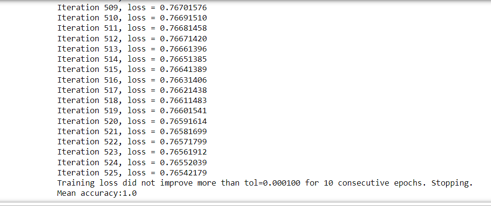
That’s all from the implementation part, and we got 100% accuracy. You can vary different parameters to view the changes.
Frequently Asked Questions
What are the limitations of perceptron? Perceptron networks have several limitations. The first one is that the output values are binary. Second, perceptrons can only classify linearly separable sets of vectors.
Can MLP be used for regression? The Multi-Layer Perceptron algorithms support both regression and classification problems. It is also called artificial neural networks.
What’s the use of bias in MLP? The bias can be thought of as how flexible the perceptron is. It is similar to the constant b of a linear function y = ax + b. It allows us to move the line-up and down to better fit the prediction with the data.
Key Takeaways
Let us brief the article.
Firstly we saw the introductory part of MLP, and then we learned why we need MLP and lastly, we saw the implementation part of MLP in two different ways, first using simple NumPy and pandas, and secondly, using sklearn.
Well, that’s one of the fundamental algorithms of neural networks. However, with Multilayer Perceptron, horizons are expanded, and now this neural network can have many layers of neurons and is ready to learn more complex patterns.


 32+ registered