L1 and L2 regularisation

Introduction

We have studied various deep learning and regression algorithms, but we missed out on an important concept, i.e., regularisation. Regularisation is a group of techniques that are used to prevent overfitting. Overfitting occurs when a model describes the training set but cannot generalise well over new inputs. In this article, we will study the various techniques used in regularisation.

Also Read About, Resnet 50 Architecture

Types of Regularisation

There are mainly three types of Regularisation:

• L1 or Lasso Regularisation
• L2 of Ridge Regularisation
• Dropout Regularisation

Our primary focus will be on L1 and L2 regularisation. You can visit this article to study Dropout regularisation. 

Also, a prior understanding of linear regression is essential; therefore, you can visit Introduction to Linear Regression  and Linear Regression: Theory and code article to brush up on your knowledge.

L1 Regularisation

Let us understand this with an example. Assume that the dataset has two features: salary and experience. Based on the years of experience, we have to predict the salary. Now, let's say that our training dataset has only two values. Therefore, the best-fit line of linear regression will pass through both points.

Hence the cost function or the sum of residual will be 0. Now to test the data:

We can see the test dataset is overfitted. Therefore, we use L1 and L2 regularisation to overcome the overfitting situation. 

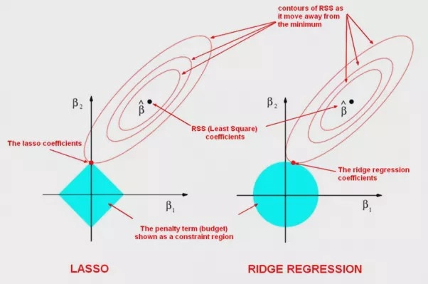
In L1 regularization, we reduce the cost function by adding the absolute value of the magnitude of the weights of various features. The mathematical representation is

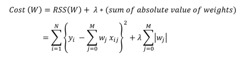
Source: Link

The L1 regularisation focuses on reducing the steepness of the best-fit line to zero, which is used to reduce the value of the cost function. That results in more accurate outputs. Apart from that, it is also used in feature selection. When the steepness is zero, there are weights whose values are zero; those features can be excluded from the data for prediction. The process of cross-validation decides the value of lambda.

Sample code 

#importing necesary libraries
import numpy as np
import matplotlib.pyplot as plt
from sklearn import linear_model
from sklearn import datasets
#importing the dataset
X, y = datasets.load_diabetes(return_X_y=True)
print("Computing regularization path using the LARS ...")
_, _, coefs = linear_model.lars_path(X, y, method="lasso", verbose=True)
xx = np.sum(np.abs(coefs.T), axis=1)
xx /= xx[-1]
#plotting the graph
plt.plot(xx, coefs.T)
ymin, ymax = plt.ylim()
plt.vlines(xx, ymin, ymax, linestyle="dashed")
plt.xlabel("|coef| / max|coef|")
plt.ylabel("Coefficients")
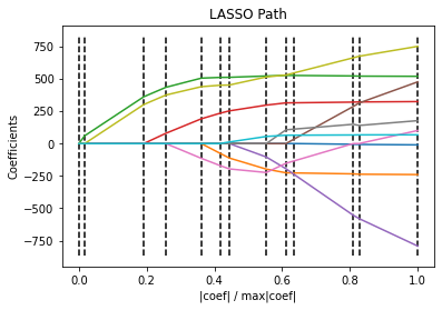
plt.title("LASSO Path")
plt.axis("tight")
plt.show()

You can also try this code with Online Python Compiler

Run Code

Output:

L2 regularisation

L2 regularisation is responsible for dealing with multicollinearity problems. It is used only to reduce the cost function by adding the square of the weights. 

The L2 regularisation also focuses on reducing the steepness and the sum of residuals. It minimizes the square of weights near zero but never equal to zero. The mathematical representation is

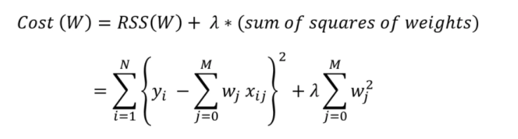
Source: Link

In L2 regularisation as well the process of cross-validation decides the value of lambda.

Sample Code

#importing necessary libraries
import numpy as np
import matplotlib.pyplot as plt
from sklearn import linear_model
# X is a 10x10 matrix
X = 1.0 / (np.arange(1, 11) + np.arange(0, 10)[:, np.newaxis])
y = np.ones(10)
# Compute paths
n_alphas = 200
alphas = np.logspace(-10, -2, n_alphas)
coefs = []
for a in alphas:
    ridge = linear_model.Ridge(alpha=a, fit_intercept=False)
    ridge.fit(X, y)
    coefs.append(ridge.coef_)
# Display results
ax = plt.gca()
ax.plot(alphas, coefs)
ax.set_xscale("log")
ax.set_xlim(ax.get_xlim()[::-1])  # reverse axis
plt.xlabel("alpha")
plt.ylabel("weights")
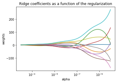
plt.title("Ridge coefficients as a function of the regularization")
plt.axis("tight")
plt.show()

You can also try this code with Online Python Compiler

Run Code

Output: