Table of contents
1.
Introduction
2.
Creating Forests of Stumps: AdaBoost
3.
Mathematical intuition behind AdaBoost
4.
FAQs
5.
Key takeaways
Last Updated: Aug 13, 2025

Understanding AdaBoost

Author aniket verma
0 upvote
Career growth poll
Do you think IIT Guwahati certified course can help you in your career?

Introduction

We will begin our discussion with how to combine AdaBoost with decision trees and Random Forests because that is the most common way of using AdaBoost. So, if you are new to decision trees or Random Forests, check it out first. So let’s start by using decision trees and random forests for explaining the concepts behind AdaBoost.

In random forests, each time you make a tree, you make a full-sized tree.


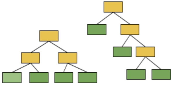
Some trees can be bigger than others, but there is no other predetermined maximum depth. The Forest of trees made with AdaBoost contains only one node and two leaves.


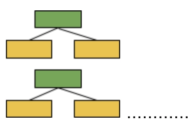
As you can see, the above figures have only one node and two leaves in them. A tree has one node and two leaves are called a stump. The above figure can better be described as a forest of stumps rather than trees. Stumps can’t make accurate classifications. For example, if we are using this data for determining if someone had heart disease or not.

Chest pain Good blood circulation Blocked arteries Weight Heart disease
No No No 125 No
Yes Yes Yes 180 Yes
Yes Yes No 210 No
Yes No Yes 167 Yes


A full-sized decision tree is responsible for taking advantage of all four variables that we measured(chest pain, good blood circulation, blocked arteries, weight, heart disease) for making a decision.


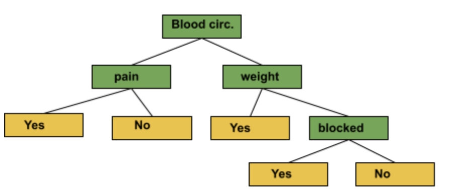
But, a stump uses only one variable for making a decision. Thus, stumps are technically “weak learners”. However, that’s the way AdaBoost likes it, and it’s one of the reasons why they are so commonly combined. Now, let’s come back to the random forest.
In a Random Forest, each tree provides an equal vote on the final classification. But in a forest of Stumps made with AdaBoost, some stumps get more say in the final classification than others. 

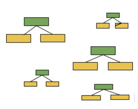
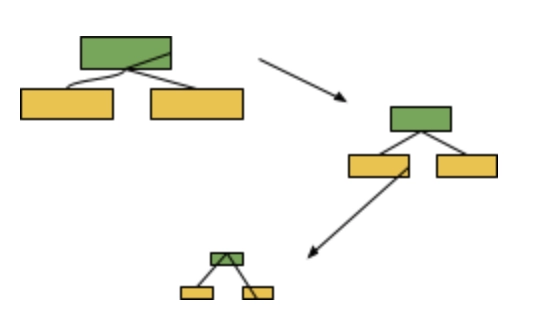
In this illustration, the larger stumps get more say in the final classification than the smaller stumps.
Lastly, each decision tree in a Random Forest is made independently. In other words, 
 

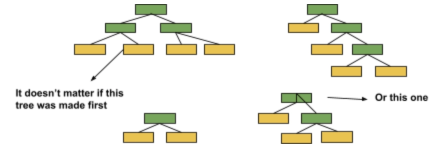
In contrast, in a Forest of Stumps made with AdaBoost, the order is important. The errors that the first stump makes influence how the second stump is made and the errors that the second stump makes influence how the third stump is made and so on.

The three ideas behind AdaBoost are:

  • AdaBoost wraps a lot of “weak learners” to make classifications. The weak learners are always stumps.
  • Some stumps get more say of proportion in the classification than others.
  • Each stump is made by considering the previous stump’s mistake into account.

Now let’s dive into the nitty-gritty details of how to create a Forest of stumps using AdaBoost.

Creating Forests of Stumps: AdaBoost

First, let’s start with some data:

Chest pain Blocked arteries Patient weight Heart disease
yes yes 205 yes
No Yes 180 Yes
Yes No 210 Yes
Yes Yes 167 Yes
No Yes 156 No
No Yes 125 No
Yes No 168 No
Yes Yes 172 No


Now, we will be creating a forest of stumps using AdaBoost for predicting whether any patient has heart disease. The decision will be based on the patient’s chest pain, blocked artery status, and weight. For that first give each sample a weight.

NOTE: the sample weight is different from the Patient’s weight. At the start, all samples will get the same weight that is 1Total number of samples.

Sample weight
1/8
1/8
1/8
1/8
1/8
1/8
1/8
1/8


In this case, 1total number of samples= ⅛. And, hence making all of them fairly important. 

After the creation of the first stump, the weights will change for guiding us on how the next stump will be created. First of all, make the first stump of the forest. This is done by finding the variable that does the best job in the fields of chest pain, blocked arteries or patient weight. As all the sample weights are the same, we can ignore that. Let’s start by seeing how well Chest pain classifies the samples.


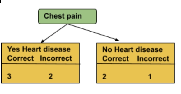
Here, of the 5 samples with chest pain, 3 were correctly classified as having a heart disease and 2 were incorrectly classified. Of the 3 samples without chest pain, 2 were correctly classified as not having heart disease and 1 was incorrectly classified. Now, for blocked arteries, we get:

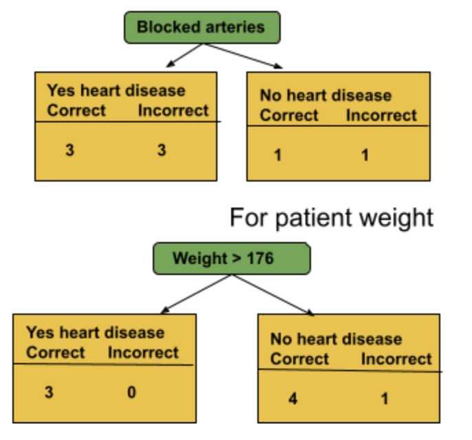
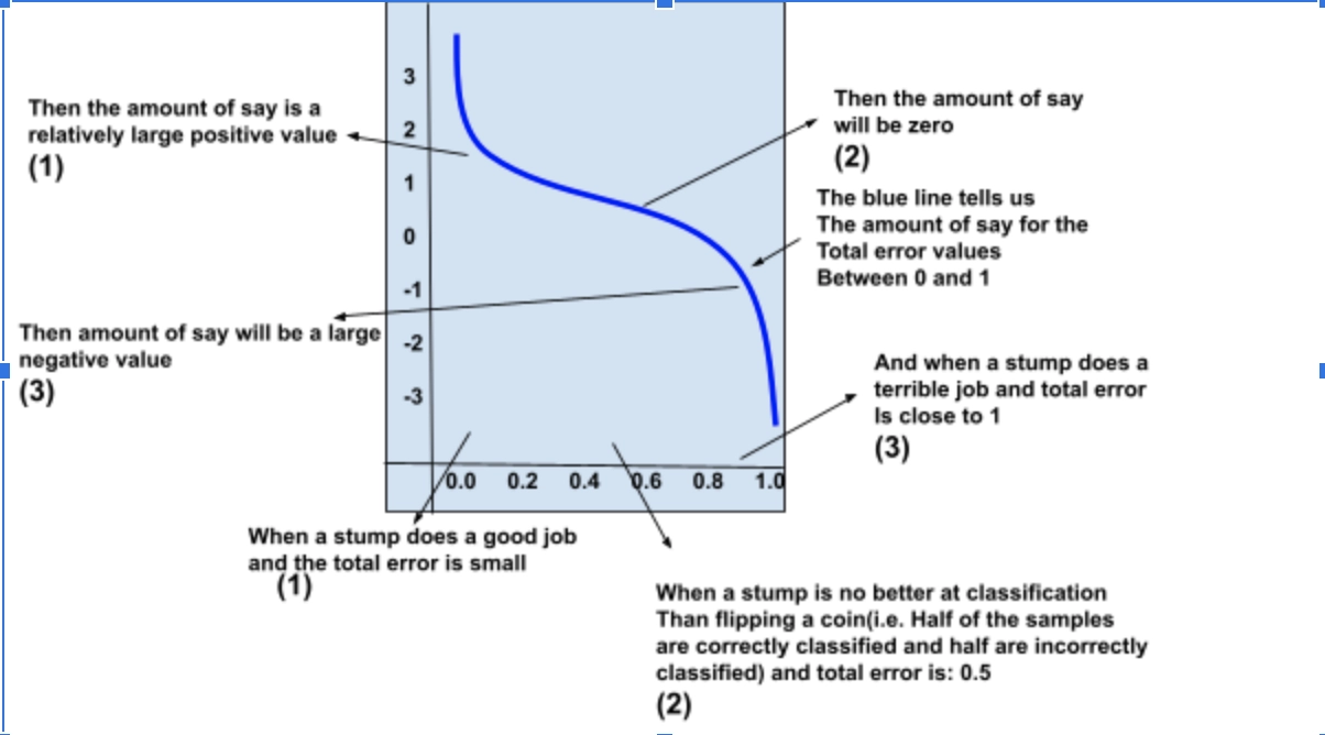
Now, we calculate the Gini Index for the three stumps. For chest pain, the Gini Index is 0.47, for blocked arteries: 0.55, and for weight: 0.2. We figure out that, the patient weight has the lowest Gini index and it will be our first stump. Now we need to determine how much say this stump will have in the final classification.

Yes Yes 167 Yes 1/8


According to the stump, even if this patient weighs less than 176, they don’t have heart disease, which is incorrect. The total error is constituted with the sum of all weights related to the incorrectly classified samples. For this case, it is ⅛.

Note: Because all the sample weights add up to 1, the Total error will always be between 0, for a perfect stump and 1, for a horrible stump.

Mathematical intuition behind AdaBoost

We use the total error to determine the amount of say this stump has in the final classification with the final formula:

Amount of say = ½ log(1-total error)/total error


For patient weight>176, the Total Error is ⅛, so:

Amount of say = ½ log(1-⅛ )/ ⅛

                        = ½ log(7)

                        = 0.97

Now, that we have worked out how much say this stump gets when classifying a sample. Let’s work out how much say the chest pain stump would have had if it had been the best stump. Chest pain made 3 errors. So:

Total error = ⅛ + ⅛ + ⅛

                 = ⅜ 

Now, we will plug ⅜ into the formula for the amount of say and do the math:

Amount of say = ½ log(⅞ ) / ⅜

                        = ½ log (7/3)

                        = 0.42


Now, we know how the sample weights for the incorrectly classified samples are used to determine the Amount of say each stump gets. Now, it is necessary for learning how to modify the weights which helps in making the next decisions. Let’s go back to the first stump we made. When we created the stump, all of the sample weights were the same and which means we did not emphasize the importance of classifying the sample. 


Yes Yes 167 Yes 1/8

But as this stump was incorrectly classified in this sample. It is necessary for the next stump to correctly classify it by enhancing its sample weight and reducing all of the other sample weights. First, increase the sample weight for the incorrectly classified sample. The formula we will use to increase the sample weight for the sample that was incorrectly classified:

New sample weight = sample weight X eamount of say

                                  = ⅛ x eamount of say

We plug in the sample weight from the last stump. 

New sample weight = sample weight X eamount of say

                                  = ⅛ e0.97

                                  = ⅛ X 2.64

                                 = 0.33

 This means the new sample weight is 0.33, which is more than the old one(i.e. ⅛ = 0.125). Now, decrease the sample weights for all of the correctly classified samples. The formula looks like this:

New sample weight = sample weight X e- amount of say

The big difference is the negative sign in front of the amount of say.

In this example, new sample weight = ⅛ X e-0.97

                                                          = ⅛ X 0.38 = 0/05.

Here, the new sample weight is 0.05( which is less than the old one i.e. 0.125).

The new sample weights column looks like this:

New sample weight
0.05
0.05
0.33
0.05
0.05
0.05
0.05
0.05


Right now, if you add the new sample weights, you will get 0.68.

Normalized weig.
0.07
0.07
0.07
0.49
0.07
0.07
0.07
0.07


Now, when we add up the new sample weights, we get 1. Now, we will use the modified sample weights for making the second stump.

If the number is lying between 0 and 0.07, then we would put this sample into the new collection of samples. And if the number is between 0.07 and 0.14(0.07 + 0.0.7 = 0.14), then we would put this sample into the new collection of samples. If the number is lying between 0.14 and 0.21(0.14 + 0.07) = 0.21, then we would put this sample into the new collection of samples. And if the number is lying between 0.21 and 0.70 (0.21 + 0.49 = 0.70) then we would put this sample into the new collection of samples.

Imagine the first number I put is 0.72. Then I would put this sample into my new collection of samples. Similarly, put other values into the new data set.

Chest pain Blocked arteries Patient weight Heart disease
No yes 156 No
Yes Yes 167 Yes
No Yes 125 No
Yes Yes 167 Yes
Yes Yes 167 Yes
Yes Yes 172 No
Yes Yes 205 Yes
Yes Yes 167 Yes


If you look carefully, you will find out that, 1 sample was added to the new collection of samples 4 times, reflecting its larger sample weight. Since the misclassified sample has more weight than others, it is more likely to enter into the new data set than others. We will be using this new data set to train our model. The above steps will be repeated until all the samples get correctly classified.

FAQs

  1. Why is AdaBoost also called Adaptive Booting?
    AdaBoost is also called Adaptive Boosting because weights get reassigned after every instance with the incorrectly classified weights.
     
  2. Is AdaBoost better than XGBoost and Random Forests?
    No, XGBoost and Random Forests are far better than AdaBoost. AdaBoost is not a time-optimized algorithm and performs terribly when irrelevant features are included in the time series analysis of bike-sharing. AdaBoost is a slow process and is not suitable for overfitting or high variance.

Key takeaways

In this article, we have learned about AdaBoosting and the Mathematical intuition behind it. Keeping the theoretical knowledge at our fingertips helps us get about half the work done. To gain complete understanding, practice is a must. To achieve thorough knowledge on machine learning you may refer to our machine learning course.

Live masterclass